

ポイント
- TSS enables analysts to detect recurring shapes and motifs in time-series data. This is especially valuable in volatile crypto markets, where past behaviors often repeat under similar conditions.
- TSS helps uncover signals by comparing historical and current data "shapes" to identify potential inflection points.
- KDB-X can handle both overlapping data windows and multi-day patterns, providing deeper insights into long-term trends.
Digital assets, such as Bitcoin (BTC), are well-known for their dramatic price fluctuations. In just a matter of hours, the market can pivot from euphoria to panic, with sharp rallies followed by swift corrections. For many, this volatility is a source of risk, but it can also be seen as an opportunity, especially when historical patterns begin to repeat.
Unlike traditional markets, which are regulated, mature, and relatively liquid, the crypto market is still evolving. Trading takes place 24/7 across fragmented exchanges with lower liquidity, making it susceptible to outsized movements from relatively small trades. When coupled with high leverage and real-time reactions to news and social media sentiment, price action in digital assets often seems chaotic and unpredictable.
Yet despite this chaos, market behavior often falls into familiar rhythms. Rallies build in stages, corrections follow predictable patterns, and “shapes” of movement tend to precede key inflection points.
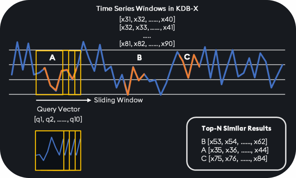
In this blog, I will demonstrate how Temporal Similarity Search (TSS) in KDB-X can help identify these “shapes” of time series data, uncovering similar patterns and recurring motifs, and how dynamic querying can enable analysts to better understand market behavior in real time.
If you would like to follow along, you can do so by downloading and installing the KDB-X Community Edition here and a sample Bitcoin dataset from Kaggle. You can also follow the full tutorial on GitHub.
Load and prepare data
From a q session, we load the ai-libs initialization script:
.ai:use`kx.aiNext, we will load three one-minute datasets (BTC, ETH, and LTC) into table memory:
tab:(" *SFFFFF";enlist ",") 0: `$":gemini_BTCUSD_2020_1min.csv";
tab,:(" *SFFFFF";enlist ",") 0: `$":gemini_ETHUSD_2020_1min.csv";
tab,:(" *SFFFFF";enlist ",") 0: `$":gemini_LTCUSD_2020_1min.csv";
Once done, we parse and clean the time column, then reorder and sort the table so that we can save our data to disk, partitioning by date:
time:sum@/:(("D";"N")$'/:" " vs/: tab`Date);
tab:`time xcols update time:time from delete Date from tab;
tab:`time xasc `time`sym`open`high`low`close`volume xcol tab;dts:asc exec distinct `date$time from tab;
{[dt;t]
(hsym `$"cryptodb/",string[dt],"/trade/") set .Q.en[`:cryptodb] `time xasc select from t where dt=`date$time;
}[;tab] each dts;
.Q.chk[`:cryptodb];
delete tab from `.;
.Q.gc[];Finally, we’ll load the on-disk data back into our process:
.Q.lo[`:cryptodb;0;0];We can validate our work by performing a simple lookup:
first select from trade where date=first date, i=0date | 2020.01.01
time | 2020.01.01D00:00:00.000000000
sym | `sym$`BTCUSD
open | 7165.9
high | 7170.79
low | 7163.3
close | 7163.3
volume| 0.00793095As we can see, the first record returned highlights a one-minute snapshot of BTC/USD trading on January 1st, 2020, including the timestamp, price range (open, high, low, close), and traded volume.
Perform TSS
With our data partitioned, we can begin searching for patterns of interest. In this example, we are going to search for closing prices that fall and rise in a V-pattern. To achieve this, we will create a V-shaped float vector and a pattern length of 64:
q:abs neg[32]+til 64;
k:10000;
For data that is non-continuous in time across date partitions, such as the NYSE, which doesn’t have 24-hour trading days, analysts are not typically interested in pattern matches that cross the date boundary. However, for markets that trade continuously across midnight, such as BTC, they may wish to find patterns that span multiple partitions, which means they may need to account for patterns in the overlap.
We will demonstrate both cases.
Query data
Let’s perform a series of queries to test our deployment. First, we will perform TSS on each daily partition, identifying where the target V-shape is best matched within that day’s close prices:
t:select {a:.ai.tss.tss[x;q;k;`ignoreErrors`returnMatches!11b];a@\:iasc a[1]} close by date from trade where sym = `BTCUSD;The starting rows of each match are pulled from the table:
res:select from trade where sym=`BTCUSD, {[x;y;z] a:x[z;`close;1]; $[all null a;y#0b;@[y#0b;a;:;1b]]}[t;count i;first date];The data is then flattened using ‘ungroup’, with two new columns, ‘dist’ and ‘match’, being populated with the distances and matching values from the search. Finally, the data is filtered to retrieve only the rows with the smallest distance values, which are considered the best matches:
d:(0!t)`close;
res:res,' ungroup ([] dist:d[;0]; match:d[;2]);
res:`dist xasc select from res where i in k#iasc dist;
date time sym open high low close volume dist match ..
---------------------------------------------------------------------------------------------------------------------..
2020.12.08 2020.12.08D12:11:00.000000000 BTCUSD 18842.04 18842.04 18841.2 18841.2 0.05202422 2.227005 18841.2 188..
2021.01.28 2021.01.28D20:14:00.000000000 BTCUSD 32925 32961.79 32925 32956.85 6.052956 2.298247 32956.85 329..
2020.12.08 2020.12.08D12:10:00.000000000 BTCUSD 18848.79 18848.79 18841.29 18842.04 0.1091669 2.319017 18842.04 188..
2020.11.04 2020.11.04D02:13:00.000000000 BTCUSD 13857.96 13891.4 13857.96 13891.4 0.4292499 2.341793 13891.4 138..
2020.02.23 2020.02.23D21:33:00.000000000 BTCUSD 9905.39 9905.39 9905.39 9905.39 0 2.353222 9905.39 990..
2020.02.23 2020.02.23D21:34:00.000000000 BTCUSD 9905.39 9905.39 9902.59 9902.66 0.08768819 2.437255 9902.66 990..
2020.12.08 2020.12.08D12:12:00.000000000 BTCUSD 18841.2 18841.2 18840 18840 0.01363459 2.4405 18840 188..
2021.01.13 2021.01.13D09:19:00.000000000 BTCUSD 34930.64 34987.76 34930.64 34987.76 0.001133045 2.45972 34987.76 350..
2021.01.28 2021.01.28D20:13:00.000000000 BTCUSD 32908.97 32925 32882.39 32925 7.625257 2.470088 32925 329..
2021.01.28 2021.01.28D20:15:00.000000000 BTCUSD 32956.85 32976.23 32949.08 32949.09 11.53418 2.470146 32949.09 329..What you have now is the k top matches of the V-shape pattern amongst all the dates in the HDB. The top row is the top match, since it has the lowest distance. The match column contains the subset of consecutive closing prices that exhibit the V-shape that day.
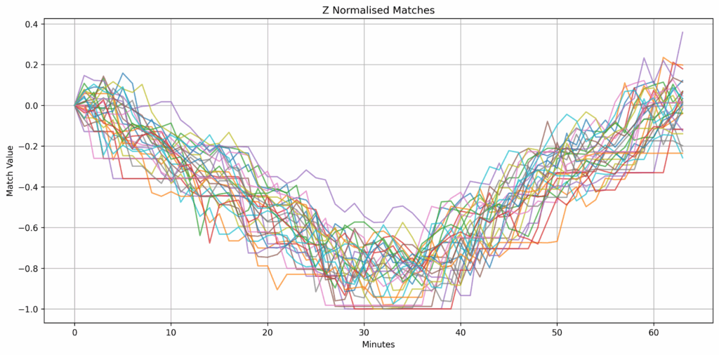
Plotting the z-normalized results reveals our top 30 closest matches
We can also search across the overlap of dates to see if TSS can detect patterns that may begin in one partition and continue into the next:
ovl:(0N;2*count[q])#count[q]_select from trade where sym=`BTCUSD, (i in count[q]#i) | (i in neg[count[q]]#i);
ovltss:.ai.tss.tss[;q;k;`ignoreErrors`returnMatches!11b] each ovl[;`close];
Finally, we can consolidate the two searches by filtering the ovltss results:
maxTopK:max res`dist;
better:where@'ovltss[;0]<maxTopK;
betterOverlap:raze ovl@'ovltss[;1]@'better;
Match data and distance data are consolidated into two separate lists with a new table called betterOverlapFull, which combines the betterOverlap data with dist and match into a single table:
match:raze ovltss[;2]@'better;
dist:raze ovltss[;0]@'better;
betterOverlapFull:betterOverlap,'([] dist:dist; match:match);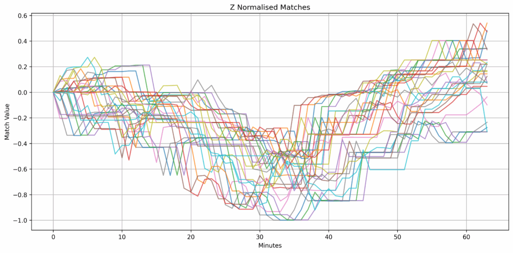
Missed matches when overlap is not considered
This process is designed to refine the results, ensuring that only the best matches are kept, and relevant information is combined into a final table, sorted for the final output res that contains the top k closest matches sorted by distance:
res:k#`dist xasc res,betterOverlapFull;Working with time-series data, especially in crypto, demands more than just storing and retrieving records. You need the ability to uncover patterns, trends, and behaviors hidden across massive datasets. In this tutorial, we explored how to do exactly that using Temporal Similarity Search (TSS). Whether you’re looking for trends within a single day or across partition boundaries, the techniques shown here, including overlap handling and symbol filtering, ensure you won’t miss critical insights.
If you enjoyed this blog and would like to explore other examples, you can visit our GitHub repository. You can also begin your journey with KDB-X by signing up for the KDB-X Community Edition, where you can test, experiment, and build high-performance data-intensive applications with exclusive access to continuous feature updates.