


Key Takeaways
- On our Intel Xeon server with 500+ GB memory, KDB-X was the only engine that answered all 84 queries. Polars, DuckDB, embedded ClickHouse (chDB) and Pandas — loading the exact same data — were killed by the OS for using too much memory. DuckDB did not survive the full data size even on the AMD box, with more than a terabyte available
- Where memory was not the binding constraint, KDB-X was the fastest solution overall. The runner-up, Polars, is 18× slower on the geometric mean of per-query ratios; embedded ClickHouse 88× and Pandas 246×. The gap widens as the data grows.
- Expressiveness is not a cosmetic concern. Because q treats dictionaries as mappings, operations that need a join or a window function in SQL are a plain function application in q-sql.
- Implementing the same 84 queries in six engines produced a long list of rough edges. This post collects the ones we think are worth knowing about before you commit to an engine.
We introduced and open sourced the KX NYSE TAQ benchmark in June 2026. It gained attention quickly, and — pleasantly — not only from our own users: engineers and maintainers behind several of the compared engines got in touch, reviewed our implementations and suggested improvements. That openness is the reason we are reasonably confident the comparison is fair.
In August 2026 we published our own measurements, taken on hardware our partners provided, and to make them explorable we built a dashboard modelled on ClickBench, the de facto industry standard for presenting database benchmark results. The second post of this series is a tour of it.
The dashboard answers precise questions well. Which engine is fastest at as-of joins on a single instrument, at 16 threads, on the AMD box? Two clicks. What it does not do is tell you the story. Reading 84 queries across sixteen solutions, three thread counts and three data sizes, and coming away with a conclusion, is work. This post is our attempt at that story: what stood out in the numbers, and what we learned from actually writing and rewriting these queries in six engines.
Everything below refers to benchmark.kx.com, where you can reproduce any chart we show, and to two machines: a dual-socket AMD EPYC 9575F (Turin, 128 cores, 2266 GB) and a dual-socket Intel Xeon 6738P (64 cores, 502 GB). Both have two NUMA nodes, and we pin the benchmark process to the first one, so a run sees about half of the cores and half of the memory listed here. Hardware details are one hover away on the dashboard.
Usability
Before speed, a more basic question: does the query return at all?
Polars, DuckDB, ClickHouse (chDB) and Pandas all hit the memory limit on the Intel Xeon box — not at the full data size, but at a smaller size (SIZE=large). Every KDB-X solution ran through the whole query set without trouble:
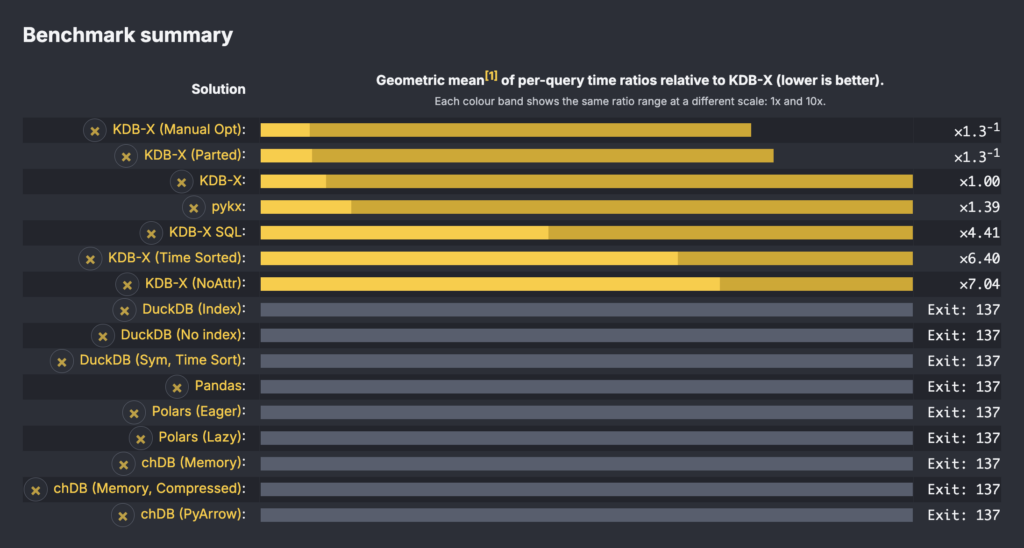
Exit: 137 is the OOM killer: 128 + 9, the process was terminated by SIGKILL because the machine ran out of memory. All seven KDB-X-based solutions in that chart, the SQL interface and pykx among them, stayed inside the budget. We pin the benchmark process to the first NUMA node, so the memory actually available on this box is not 502 GB but roughly half that, about 251 GB.
Memory need is a property of the solution, not of the server, and running the same large configuration on the AMD box — same NUMA pinning, but half of 2266 GB to play with rather than half of 502 — shows why the Intel run went the way it did. These are max resident set sizes as time -v reports them:
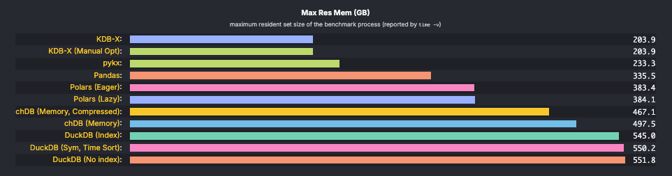
Read that against the 251 GB an Intel node offers and the Exit: 137 column explains itself. KDB-X at 204 GB and pykx at 233 GB are the only two that fit. Pandas needs 336 GB for the same rows, Polars 384, chDB up to 498, and the three DuckDB configurations between 545 and 552. None of them could have finished on the Intel box whatever the query set had been — nothing about their query execution was tested there at all.
DuckDB is the extreme case, needing 2.7 times what KDB-X does.
When a solution requires nearly three times the memory of another to answer the same question, that is a deal breaker for a lot of production systems, whatever the timings say.
It also decides where analysis can happen. Fitting the working set in a fraction of the memory is what lets a quant do genuine exploratory work in production, against the live dataset, rather than against a copy. The alternative pattern — pull a subset out of the system of record into a separate process for the last mile of wrangling — is widespread enough to be treated as established best practice, but a good part of the reason it is established is that some of these tools cannot do anything else. Pandas only ever works on a fully materialized in-memory frame, and the chart above shows it is expensive even in the one mode it has. Note that both KDB-X front ends fit inside an Intel node, pykx at 233 GB included: the Python ergonomics do not cost you the ability to stay where the data is. If exploration requires extracting the data first, exploration becomes something you schedule rather than something you do.
And the copy is not a neutral cost. Every extract is a fork of the truth: it is a subset, taken at a moment, under filters that live in whoever’s script pulled it. Two quants asking the same question of the same system get different answers because they cut different slices; a result from last quarter cannot be reproduced because the extract that produced it is gone, or has been quietly corrected upstream since. The consistency and reproducibility problems that follow are usually attributed to process, and teams answer them with more process — extract catalogues, lineage tracking, snapshot conventions. Much of that machinery exists to compensate for an engine that could not answer the question in place.
Elegance of the query language
Execution time is measurable and therefore gets all the attention. Having implemented the same 84 queries six times, we would argue the language matters at least as much, because it is the part you live with every day.
The solutions fall into three groups:
- Pythonic API — KDB-X Python (
pykx), Pandas and Polars. Method chains over dataframe objects, with the query built up as Python expressions. - SQL dialects — DuckDB, chDB and KDB-X SQL. ANSI SQL as the common core, plus each engine’s own extensions, which is where they diverge.
- q-sql — KDB-X’s third option, and neither of the above: the query sublanguage of q, an array language in which tables and row order are primitives rather than extensions. The rest of this section is largely about what that buys you.
ANSI SQL is limited enough that every engine extends it, and the extensions are where the dialects diverge. SQL is excellent for simple analyses and becomes cumbersome as the query gets more complex. Take a fill-forward on table t: replace every null with the previous non-null value in its column. In q it is one function applied to the whole table:
fills tIn SQL it is a window function, and even with DuckDB’s COLUMNS(*) shorthand — itself an extension, not standard SQL — the statement is:
SELECT time,
       LAST_VALUE(COLUMNS(* EXCLUDE time) IGNORE NULLS)
           OVER (ORDER BY time ROWS BETWEEN UNBOUNDED PRECEDING AND CURRENT ROW)
    FROM t
    ORDER BY time
time appears three times: once to keep it in the output, once inside the window to define what “previous” means, and once at the end because the row order of the result is otherwise not guaranteed. In q, “previous” is the order the rows are already in.
Query 56 is another example. Find the largest trades on every exchange. The q-sql solution:
select from trade where size = (max;size) fby exfby applies an aggregate within groups and compares it back against the ungrouped rows, which is exactly the shape of the problem. In SQL you reach for a window function, a subquery, and — because SQL has no inherent row order — an explicit rowid to restore it:
SELECT * EXCLUDE (max_size, rowid) FROM
    (SELECT *, rowid, MAX(size) OVER (PARTITION BY ex) AS max_size FROM trade)
    WHERE size = max_size
    ORDER BY rowid
Tables only
ANSI SQL knows about tables and functions, and nothing else. That constraint pushes some perfectly simple logic into a more elaborate shape than it deserves.
Take a simplified benchmark query: the maximum trade size per exchange. q-sql and SQL are near-identical here:
q)select maxsize: max size by ex from trade
ex| maxsize
--| -------
A | 744875
B | 30000
C | 72000
D | 8248817
G | 18100
...
SELECT ex, MAX(size) AS maxsize FROM trade GROUP BY ex
Now tweak the requirement. Report the maxima by exchange name rather than exchange code. The NYSE TAQ specification defines a one-to-one mapping between the two, and in q we keep it in a dictionary called exnames. The dictionary goes straight into the query:
q)select maxsize: max size by exName: exnames ex from trade
exName                            | maxsize
----------------------------------| -------
                                  | 161000
Cboe BYX Exchange                 | 50000
Cboe BZX Exchange                 | 1078984
Chicago Stock Exchange            | 2300000
FINRA Alternative Display Facility| 8248817
...
The change in the requirement produced a proportional change in the code: one dictionary name, zero noise. KDB-X users know that kdb+ descends from APL, developed by the mathematician Kenneth E. Iverson, and in mathematics dictionaries and functions are both just mappings. q keeps that identity, so anything you can apply, you can apply here.
SQL has no dictionaries, so the mapping becomes a two-column table, the lookup becomes a left join, and both tables need aliases:
SELECT COALESCE(e.name, '') AS ex, MAX(t.size) AS maxsize
    FROM trade t LEFT JOIN exnames e ON t.ex = e.ex
    GROUP BY e.name
Note the COALESCE. A left join produces NULL for an exchange code missing from exnames, and that NULL has to be handled explicitly to match what the dictionary lookup gives you for free. Engineering workarounds and unnecessary noise on top of a simple problem.
KDB-X SQL, incidentally, sidesteps this: .s.F and .s.fx allows injecting any q mappings — including dictionaries — into the SQL interface as scalar functions, so the query reads GROUP BY exnames(ex). The mapping stays a mapping.
q).s.F[`exnames]: .s.fx exnames;
q)s)SELECT exnames(ex), MAX(size) AS maxsize FROM trade GROUP BY ex
exnames                            maxsize
--------------------------------------------
NYSE American                      744875
NASDAQ OMX BX                      30000
NYSE National                      72000
FINRA Alternative Display Facility 8248817
...
Step dictionaries
There are more tricks in the KDB-X sleeve. Consider a simplified version of query 63, which computes statistics over custom time buckets — premarket, morning, afternoon and so on — defined by their lower bounds. A step dictionary is made for this. It is an ordinary dictionary with the sorted attribute applied, and when a key is absent it returns the value of the nearest preceding key instead of a null:
q)buckets: (0D00:00:00; 0D04:00:00; 0D09:00:00; 0D09:30:00)!`closed`preopen`open`morning
q)timeBucketsStep: `s#buckets
q)timeBucketsStep 0D06:12:43.115
`preopen
Being a mapping, it drops into a query the same way exnames did:
select cnt: count i, sum size
    by timeBucket: timeBucketsStep time
    from trade
The solution is syntactically identical to the exchange name example, which is the point: a step dictionary is just a mapping with some syntactic sugar over the lookup.
SQL gets to the same result, but the bucket table has to be joined, and because the match is “nearest preceding bound” the join is an as-of join:
sql
SELECT bucket AS timeBucket, COUNT(*) AS cnt, SUM(size) AS size
    FROM trade t ASOF JOIN timeBuckets ON t.time::TIME >= timeBuckets.bound
    GROUP BY timeBucket
    ORDER BY timeBucket
None of this is unachievable in SQL. It is just that the shortcuts KDB-X offers make the analysis more direct, and — we would say — more fun.
Speed
Query speed can be compared query by query, and the dashboard lets you do exactly that. It also lets you aggregate: pick a baseline engine, form the per-query ratios against it, and take the geometric mean over whichever subset of queries you care about. Selecting the largest data size (full) and 4 threads on the AMD Turin box gives the following, as of the time of writing (September 2026):
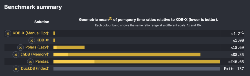
KDB-X is the fastest solution. The runner-up, Polars, is 18× slower on average. Embedded ClickHouse in its memory engine configuration is 88× slower, and Pandas 246×, better than two orders of magnitude behind. KDB-X experts can take a further 16% off the average by hand-parallelizing a handful of queries with peach — that is the KDB-X (Manual Opt) row. DuckDB was killed, despite the pinned node still offered more than a terabyte, which is why its bars are missing.
Shrinking the data brings DuckDB back into the picture, since it no longer runs out of memory:
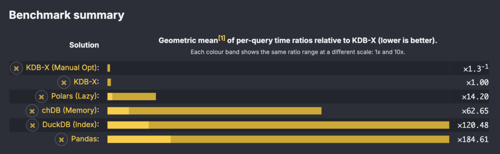
DuckDB with an index lands 120× behind KDB-X. Comparing the two charts also shows the direction of travel: Polars moves from 14.2× to 18.7×, chDB from 62× to 88×. The more data, the wider the gap in KDB-X’s favour, which is worth keeping in mind if you are evaluating an engine on a sample and planning to deploy it on a day.
Aggregates flatten things, so it is worth opening individual queries. Differences there can be substantial. For as-of join queries KDB-X is frequently more than two orders of magnitude ahead of any other engine, and against Pandas the ratio reaches 15,461 on query 84, which joins ten minutes of pre-close trades to their prevailing quotes — 284 seconds against 24 milliseconds. chDB is worse still: it does not finish two of the as-of joins at all within our time limit.
Query 46 is a second example, a size-weighted bid and offer price for a thousand infrequently traded instruments. Taking SIZE=xlarge on 4 threads, the one configuration where every engine survives, KDB-X answers in 11 ms. Polars needs 1.8 s (×166), Pandas 18.8 s (×1,749), and DuckDB with an index 201.6 s — over four orders of magnitude behind KDB-X on a query that is, by the benchmark’s own classification, simple.
KDB-X Python (pykx)
pykx costs almost nothing where it matters. Across the queries in which KDB-X itself takes more than 10 ms, pykx is on average at the same speed as q expressions in a q session, which is what you would expect from two front ends to the same engine. What pykx adds is a fixed cost of two to three milliseconds per call, invisible on a six-second query and dominant on a sub-millisecond one. Query 81, an as-of join against a single infrequently traded instrument, is the extreme case: at SIZE=full KDB-X answers in 146 µs and pykx in 3.0 ms. Those sub-millisecond queries are what pushes the pykx aggregate to ×1.39 in the Intel chart above rather than to ×1.00, and it is worth reading that row as a per-call latency floor rather than as a 39% throughput penalty. If your workload really is sub-millisecond point lookups issued one at a time, measure it yourself; for anything else, choosing Python over q costs you nothing in throughput.
Issues with the engines
Nine months of implementing, reviewing and re-implementing these queries left us with notes. The following are the ones we would want to know before committing to an engine.
Polars
Polars is the strongest of the alternatives, and most of what we have to say about it is about the API rather than the engine. Pythonic dataframe code carries a lot of noise — parentheses and quotation marks everywhere — which is easiest to see side by side. Query 29, already shown in the first post, pivots the 10-minute average liquidity-weighted mid-quote by symbol for a thousand infrequently traded instruments and forward-fills the gaps.
q-sql:
fills .pvt.pivot select
    avgLiqWMid: avg ((bsize * bid) + asize * ask)
                     % bsize + asize
    by 10 xbar time.minute, sym
    from quote
    where sym in thousandInfreqInstr
Polars:
   quote
    .filter(pl.col("sym").is_in(thousandInfreqInstrs))
    .with_columns(time = pl.lit(datadate).dt.combine(pl.col("time")))
    .group_by_dynamic(index_column="time", every="10m",
                      closed="left", group_by=["sym"])
    .agg(
        ((pl.col("bsize") * pl.col("bid") +
          pl.col("asize") * pl.col("ask"))
         / (pl.col("asize") + pl.col("bsize")))
        .drop_nans().mean().alias("avgLiqWMid")
    )
    .pivot("sym", values="avgLiqWMid", index="time")
    .with_columns(pl.col("time").dt.time())
    .sort("time")
    .select(pl.all().forward_fill())
Three of those lines are not there by choice. group_by_dynamic does not accept duration types, so the time column has to be combined with the date first and stripped back to a time afterwards. And group_by_dynamic has no maintain_order parameter, so the result needs an explicit sort.
One more observation, since the dashboard exposes both: the lazy API is not a free win. At 16 threads, Polars (Eager) and Polars (Lazy) split the 84 queries roughly evenly. Query planning helps where there is something to plan, and costs where there is not.
DuckDB
- Speed, as covered above: DuckDB is well behind KDB-X, by more than two orders of magnitude on a number of queries.
- Memory: DuckDB is the hungriest engine in the comparison, 545 GB resident at
SIZE=largeagainst KDB-X’s 204 GB, and the only engine that ran out of memory on the AMD box — killed at the full data size with more than a terabyte on the pinned node. ENUMversus symbol. DuckDB’sENUMrequires the distinct values to be collected up front, so ingesting a table means a pre-pass over the data, and a value not seen during that pre-pass means altering the type. kdb+ extends its symbol mapping automatically on insert; there is nothing to plan for.- Filtering on a single enum value is not intuitive either. The obvious ANSI SQL predicate
SELECT * FROM quote WHERE sym = 'KX'compares an
ENUMcolumn against a string, andEXPLAINshows the price: the filter becomesCAST(sym AS VARCHAR) = 'KX', decoding the dictionary into strings for every row. Casting the literal into the enum keeps the comparison on the dictionary index, but works only for values the enum already contains:SELECT * FROM quote WHERE sym = 'KX'::sym_enum -- filter: sym='KX' SELECT * FROM quote WHERE sym = 'KXfoo'::sym_enum -- Conversion Error: Could not convert string 'KXfoo' to UINT8Asking for an instrument that did not trade that day is an ordinary query that should return no rows. The uncast form does exactly that, quietly; the fast form fails outright and reports the dictionary’s physical index type, which is nothing the user wrote. The predicate that is both fast and safe turns out to be a third one:
SELECT * FROM quote WHERE sym = TRY_CAST('KXfoo' AS sym_enum)TRY_CASTgivesNULLfor an unknown symbol, so the comparison is never true and the result is empty, with the same plan as the fast version.None of this arises in q, where the column holds symbols and
`KXis a symbol:select from quote where sym=`KX - Indexing is not the straightforward win it is in KDB-X, where a grouped attribute is a reliable accelerator. Compare
DuckDB (Index)andDuckDB (No index)on the dashboard and you will find queries where the unindexed configuration is substantially faster — query 51 by more than 10×. - The
timecolumn holds durations since midnight with nanosecond precision, and DuckDB’s type system does not have a comfortable home for it.INTERVALonly carries microseconds;TIME_NSandTIMESTAMP_NSdo carry nanoseconds, buttime_bucketdoes not acceptTIME. Once you settle onTIMESTAMP_NS, how should the very first benchmark query — all quotes before 8 AM — be written?SELECT * FROM quote WHERE time < $1 + INTERVAL '8 hours'or simply
SELECT * FROM quote WHERE time::TIME < '08:00'One is fast, the other is readable. With KDB-X the dilemma does not arise:
select from quote where time < 0D8
Embedded ClickHouse (chDB)
chDB gave us the most trouble, and the deepest problem is that it guarantees no row ordering if multiple threads are used. That is defensible in a distributed analytical engine and awkward in time-series work, where order is the data.
It gets worse in as-of joins. ClickHouse’s ASOF JOIN does not define a tie-break among rows sharing the join key, so when several quotes carry the same (sym, time) it may return any of them. The benchmark specifies the prevailing quote as the last in table order, so the tie has to be resolved explicitly with a window function on the right-hand table — which slows the query down enough that we then hand-optimized the sym filter to claw some of it back. Query 84 ends up as:
SELECT t.sym, t.time, t.price, t.size, t.stop, t.cond, t.ex, q.bid, q.ask, q.bsize, q.asize, q.cond AS quotecond
    FROM (
        SELECT sym, time, price, size, stop, cond, ex, rowid FROM {trade}
        WHERE time BETWEEN INTERVAL 980 MINUTE AND INTERVAL 990 MINUTE) t
            ASOF LEFT JOIN (
                SELECT sym, time, bid, ask, bsize, asize, cond FROM {quote}
                WHERE sym IN (SELECT DISTINCT sym FROM trade WHERE time BETWEEN INTERVAL 980 MINUTE AND INTERVAL 990 MINUTE)
                QUALIFY row_number() OVER (PARTITION BY sym, time ORDER BY rowid DESC) = 1) q
            USING (sym, time)
ORDER BY t.rowid
The q-sql solution:
aj[`sym`time;
    select sym, time, price, size, stop, cond, ex from trade where time within 0D16:20 0D16:30;
    select sym, time, bid, ask, bsize, asize, quotecond: cond from quote]
aj is a single primitive that means “prevailing value as of”, tie-break included. Note also INTERVAL 980 MINUTE against 0D16:20: the SQL has to express 16:20 as minutes since midnight, because there is no readable literal for an intraday offset.
Readability aside, chDB never finished this query at the full data size, nor at 4 or 16 threads at any size. The one configuration in which it completed — SIZE=large on 64 threads — took 7,952 seconds, a little over two hours, against 7 ms for KDB-X. A ratio of 1,096,502 is the largest single-query gap anywhere in the benchmark.
Other problems we ran into:
- No in-place sort. Sorting a table means materializing a copy, which matters when the table is hundreds of gigabytes.
- Sorting on a
LowCardinality(String)key is extremely slow. We had to convert those columns to plain strings, sort, and convert back to dictionary-encoded strings to get acceptable load times. - No
PIVOT. Queries 24 to 29 have no chDB implementation at all, which is the most direct expressiveness result in the whole benchmark: six of 84 queries are simply not expressible. - With PyArrow tables as the storage format, restricting the thread pool deadlocks the engine. A plain
SET max_threads = 16is enough: the process then hangs in a ‘futex’ wait on thread synchronization and never returns. This is why ‘chDB (PyArrow)’ on the dashboard shows results at 64 threads only, while the two ClickHouse ‘Memory’ configurations report all three thread counts. It is the one solution in the whole comparison we could not run at a restricted thread count — every other engine, chDB’s own ‘Memory’ format included, took the setting without complaint. Thread scaling is one of the more revealing dimensions of the benchmark, and for that solution we cannot measure it at all.
What is next
Everything above is reproducible. The benchmark suite is at github.com/KxSystems/NYSETAQBenchmarks, the results are at benchmark.kx.com, and the quickstart runs on a ‘tiny’ dataset that fits on a laptop with the free KDB-X Community Edition. If you think a query is unrepresentative of your workload, untick it on the dashboard and watch the aggregate move. If you think one of our implementations is suboptimal, the pull request is welcome — several of the numbers above are better than our first attempt because someone did exactly that.
The next stage of the program moves the data to disk: kdb+ against Parquet, and KDB-X against the other engines reading the same Parquet files.