What’s new in KDB-X GPU Acceleration?: Nested columns, profiling, and performance tuning

In our first blog announcing the release of KDB-X GPU Acceleration, we highlighted the ways in which leveraging the GPU module optimizes the heaviest compute operations in a KDB-X system. The fundamentals are clear: push your key columns to device, let .gpu.aj or .gpu.xasc do the heavy lifting, and bring results back only when you need them. The latest release version of this module brings several improvements across the board, including a few useful new additions worth knowing about – namely nested column support, a new profiling API, and a memory tuning knob that, in one of our benchmarks, cut runtime by up to 40%!

Nested columns: Grouping with lists of values

Until now, GPU operations worked only on flat, scalar columns. That covers the majority of tick data use cases, but it leaves out a common and useful pattern – grouping rows into lists. This is the exact type of operation when running something like select y by x from t.

The GPU module now supports this directly, with one level of nesting. The implementation deliberately favors flat data structures internally, since cache locality matters significantly for the highly parallel algorithms running on distributed multi-threaded GPU devices. That’s an implementation detail you won’t see from the q side, but it changes the current depth limit we can support, which will likely bring a lot of extra mileage. Here’s what that looks like in practice:

The q equivalent is the familiar 0!select y by x from t – results are identical (note the use of 0! as keyed tables are not yet supported). Moving averages work the same way:

Same as 0!select 3 mavg y by x from t. The pattern composes cleanly. Group by a column, apply a moving scan, get back nested lists – all happening directly on GPU until you call .gpu.from.

Profiling your GPU workloads

When a GPU pipeline is slower than expected, the problem is rarely the CUDA kernel itself. This usually stems from resource management; how memory is allocated, when kernels are launched, and where the CPU/GPU are waiting on each other. Nsight Systems is an invaluable tool that gives an excellent window into how this is working, and GPU module v2.0 makes it significantly more useful for KDB-X workflows.

If we run a small script doing a couple sums on 10,000,000 rows, we can see the first run of the query is actually slower before leveling out:

Typically, we could just start by profiling with nsys (Nsight Systems), but there is a lot going on and it’s hard to see the interesting bit:

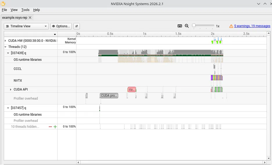
The new entry points within this module come from .gpu.profiler.start[] and .gpu.profiler.stop[], which expose cudaProfilerStart and cudaProfilerStop, respectively. Without these, profiling a q script captures everything, from q startup to data loading, and everything in-between – this ends up with a trace full of noise. Now, leveraging these APIs allows for input of exactly the code you care about, clearly visualizing the relevant bits:

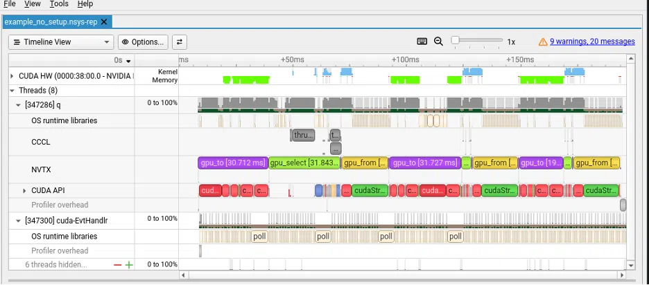
Now our trace shows only the three query executions. We cut directly into what we care about, with no startup overhead and no unrelated work.

From here, we can embed landmarks into our trace using .gpu.nvtx.start and .gpu.nvtx.end. They let you define named ranges that show up as labeled bands in Nsight Systems – we can tweak our profiler_exampleGpu.q script to add these as follows:

Using the NVTX drop down, we can visualize the range that has been inserted along with its duration:

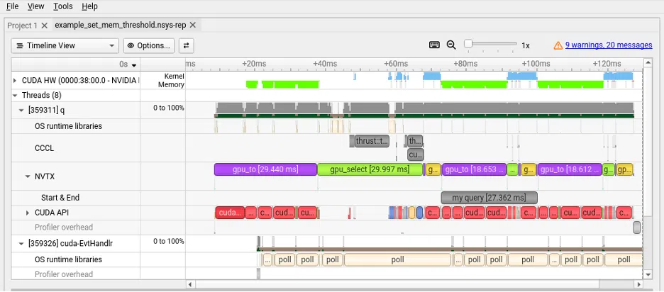
We can see the initial runs of .gpu.to and gpu.select are taking a lot longer, but that is fairly normal as the CUDA driver initializes parts of the system that can be reused. The GPU module already defines some internal NVTX ranges (specifically data transfer and select statements), so the custom ones sit alongside them in the same timeline view. When chasing a latency spike across a multi-step pipeline, being able to see exactly where your workload boundaries fall is genuinely useful.

Tuning memory release behavior

Nsight Systems clearly illustrates the above pattern where the first run of a query is slower, but that is a red herring artifact of initialization, in subsequent runs we see.gpu.from spends most of its time waiting rather than transferring data. The memory pool releases all unused memory at synchronization points, meaning every time .gpu.from syncs to return data to the CPU, the pool frees its reserved memory. The next allocation then goes back to the CUDA driver.

This is where .gpu.setMemRelThres comes into play – this function sets a ceiling on how much memory the pool retains across sync points. It doesn’t cap how much memory can be allocated; just prevents the pool from releasing memory it might need again shortly. Integrating this into the beginning of our example script, our final version (including all profiling injection changes) looks like:

This knocked nearly 40% of the runtime off! The issue of the memory pool releasing unused memory on synchronizations is rendered obsolete by setting the threshold to 20Gb, so nothing is released and the time spent on freeing memory is gone. This is also a small performance increase by avoiding going through the CUDA driver for subsequent allocations. Note that the threshold is set per device, so in a multi-GPU setup its best practice to configure each one explicitly after calling .gpu.setdev (formerly .gpu.sdev).

At very large scale, you’re trading memory overhead for allocation speed. A 20Gb threshold on a 40Gb A100 leaves plenty of room. However, on a smaller device or a workload with genuinely variable memory demands, this should be tuned accordingly.

Device utility function changes

The device management functions have been renamed to avoid confusion of sdev with standard deviation:

The behavior is identical – .gpu.cntDev[] still returns the number of available devices, .gpu.memDev[] still returns available memory, and so on. If you have existing scripts that reference the old names, update them before upgrading.

Closing Thoughts

In combination, these changes round out the GPU module in two meaningful ways. Nested column support opens up grouped aggregation patterns that were previously only supported on CPU. Plus, the profiling and memory tuning APIs give users the visibility and control to squeeze more out of the hardware you already have, without guessing at where the time is going.

The initial release set the foundation. This second iteration pulls it off the ground in meaningful ways with expanded functionality. The fastest time-series database in the world just got a whole lot faster – with additional layers to unlock its full potential by leveraging full capabilities of GPU acceleration.

Learn more about KDB-X GPU Acceleration here.

Interested in building yourself? Learn how to leverage GPU Acceleration with your current workloads in our tutorials, which can be found here.