
Co-author: Ryan Siegler
Algorithmic trading, powered by expert systems, deep learning models, and, increasingly, transformer-based generative AI, is transforming modern financial markets. From optimizing trading strategies and managing risks to enhancing portfolio performance and analyzing market sentiment, deep learning has reshaped the industry, empowering analysts to uncover hidden patterns and predict market trends with unprecedented speed and accuracy.
This four-part series will explore continuous learning using deep learning models, GPUs, and kdb+ as a data platform.
- Part 1 will look at how to use data from kdb+ to drive deep learning
- Part 2 will explore real-time inference and deploying deep learning models at your data
- Part 3 will look at implementing RAG and deep learning as a tool
- Part 4 will conclude with operationalization and visualization for deep learning
Let’s begin
The challenges of modern market analysis
An algorithmic approach to modern market analysis means emotion-free, low-latency decision-making but creates a hyper-competitive environment where alpha decays faster than ever. To stay ahead, firms must capture alpha from petabytes of high-frequency, high-volume data, including structured L2 and L3 market data, order books, execution logs, and unstructured data, such as news, social media sentiment, and financial reports.
Success depends on capturing, ingesting, processing, and acting on this data in real time without compromise. Ultra-low latency, massive scalability, and AI integration are no longer luxuries; they are the foundation for survival.
Many turn to kdb+, the industry standard in high-frequency time-series data and real-time analytics to power the data for deep learning models.
Deep learning offers advanced financial models; realizing its potential requires careful consideration. These models are susceptible to overfitting, and generalizing across diverse data requires rigorous preprocessing and thoughtful design. Therefore, best development, validation, and monitoring practices must be employed.
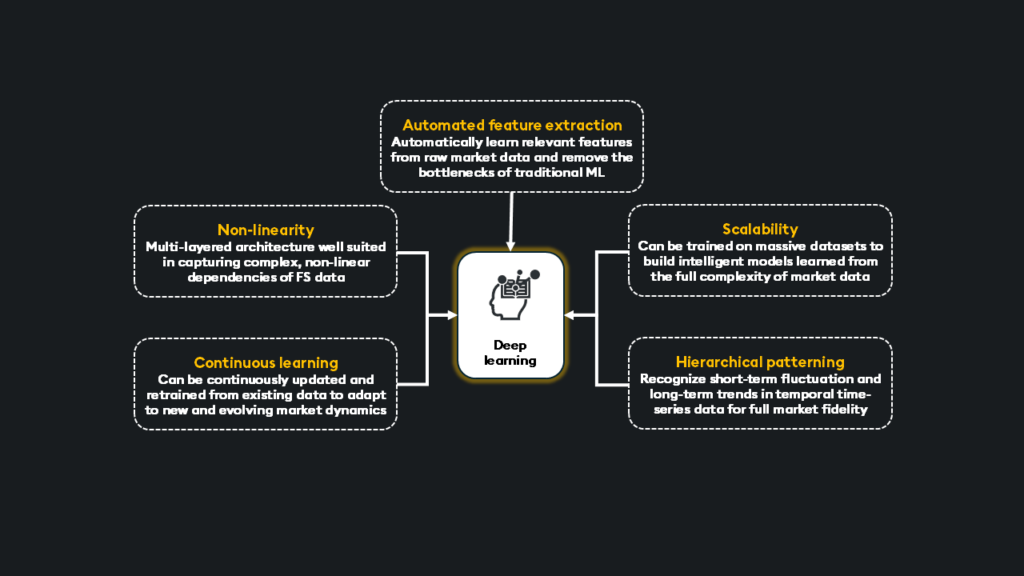
Traditional statistical methods, like linear regression or ARIMA models, rely on pre-defined assumptions like linearity and distribution but can be highly effective for specific tasks like basic risk assessment or forecasting simple time series. Machine learning models, such as random forests or gradient boosting machines (GBM), though requiring feature engineering, handle non-linearity well and often provide excellent performance in areas like credit scoring or fraud detection.
Deep learning’s power comes at a cost: computational intensity. Training complex models on petabyte-scale datasets requires significant processing power, and real-time inference demands ultra-low latency. GPUs provide the parallelism to accelerate model training and inference, reducing long-term short memory (LSTM) training from days to hours and sub-millisecond inference on streaming market data.
What technology is necessary for deep learning at scale?
A deep learning stack should provide:
Requirements:
- A high-performance data platform such as kdb+
- A deep learning framework such as PyTorch to simplify development workflows
- A GPU to expedite parallel processing at a petabyte-scale
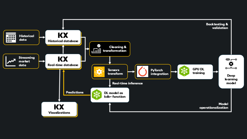
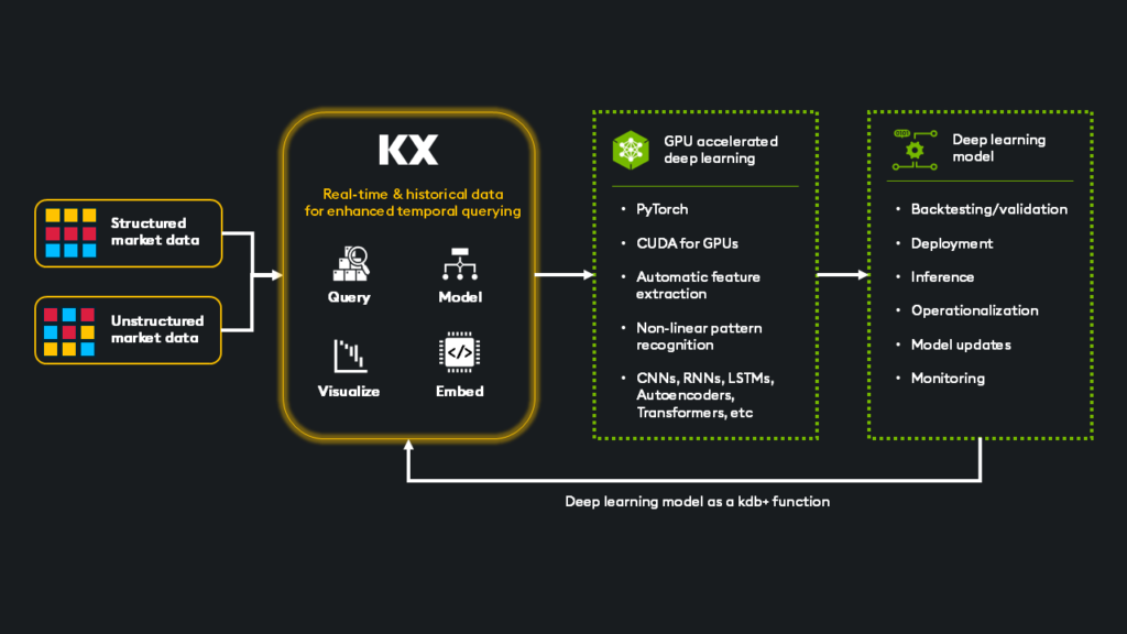
kdb+ provides an all-in-one data layer for deep and continuous learning, contributing performance enhancements in the following phases:
- Data access: kdb+ integrates historical and real-time data, combining its historical database (HDB) with a real-time tick data streaming architecture, providing a unified view of your entire data estate for model training.
- Data preparation & transformation: kdb+ enables ultra-fast data transformations necessary for preprocessing, cleaning, filtering, and feature engineering (when required) at scale. Its powerful query language (q) and PyKX (Python interface) simplify complex data manipulations and data preparation for AI workflows
- Tensor conversion: PyKX facilitates easy conversion of kdb+ data into tensors, the fundamental data structure for deep learning frameworks like PyTorch. This direct conversion streamlines the integration of kdb+ data with training pipelines and DEEP LEARNING frameworks, eliminating data format bottlenecks
For example:
import pykx as kx

kx.q.til(10).pt()  # Converts kdb+ data to a PyTorch tensor

>>> tensor([0, 1, 2, 3, 4, 5, 6, 7, 8, 9]) - Validation and backtesting: kdb+’s ability to store and rapidly query vast amounts of historical data is integral to integrated model validation and backtesting. Analysts can replay years of market data to assess model performance under various market conditions, ensuring reliability before deployment
- Real-time inference:kdb+ plays a vital role in operationalizing trained and validated deep learning models for real-time inference
- Model-to-data architecture: kdb+ allows trained models to be integrated and serve as first-class functions within the kdb+ process. This “model-to-data” architecture is highly advantageous because inference happens directly on the live, streaming data, ensuring the latest data and the lowest latency
- Filtering and processing: Before inference, kdb+ can efficiently filter and process the incoming data, sending only the necessary data to the on-GPU inference service (e.g., NVIDIA Triton, NIMs) via Inter-Process Communication (IPC)
- Direct data integration: The output from the deep learning model can be directly added to existing kdb+ tables, allowing immediate integration of inference results with other data, enabling further analysis, as-of joins, and more complex, rule-based decision-making
- GPU integration: kdb+ integrates with GPU inferencing services like NVIDIA Triton and NIMs, leveraging the power of GPUs for ultra-low latency inference on streaming market data. This tight integration ensures that trading strategies react instantly to market changes
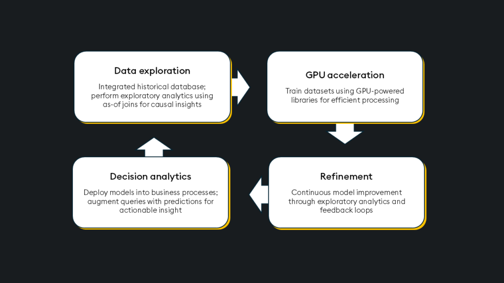
- Visualization & model updates: Once operationalized and deployed on GPU infrastructures as a first-class function in kdb+, the model ingests fresh, low-latency data. Predictions are integrated directly into the data workflow and can be visualized and used in further analysis.
Because data preparation, tensor conversion, and deep learning framework integration are already part of the pipeline, model updates (even continuous updates) are not only supported but made efficient, adapting to evolving market dynamics and avoiding significant model drift.
Deep learning framework: PyTorch
PyTorch is a leading framework for deep learning in finance. It offers a powerful combination of flexibility, GPU integration through NVIDIA CUDA, and community with the familiar Pythonic experience.
One of its key features is its dynamic computation graph architecture, which enables greater flexibility in building and experimenting with complex models. This is especially fitting for the financial domain, given market conditions can rapidly change. Furthermore, the framework’s native Python integration provides access to extensive libraries, simplifying and accelerating development.
PyTorch also supports pre-trained models and transfer learning, integrating directly with NVIDIA CUDA for GPU acceleration of model training, transfer learning, and inference. With GPUs’ parallel processing capabilities, PyTorch can significantly reduce training times for deep neural networks and accelerate inference on real-time data.
# Use PyKX to transform kdb+ data -> tensor, and PyKX to load the tensor to a GPU
import torch
import pykx as kx

# Check if CUDA is available
if torch.cuda.is_available():
    device = torch.device("cuda")  # Use the first available GPU
    # Or specify a specific GPU if you have multiple
    # device = torch.device("cuda:0") # For GPU 0
    # device = torch.device("cuda:1") # For GPU 1, and so on.
else:
    device = torch.device("cpu")

# Create a tensor using PyKX
my_tensor = kx.q.til(10).pt()

# Move the tensor to the GPU
my_tensor = my_tensor.to(device)
GPUs
With their general-purpose design, CPUs struggle with complex, high-frequency data streams generated by financial markets.GPUs, however, are optimized for the parallel computations inherent in neural networks and designed to efficiently handle matrix multiplications, convolutions, and other operations involved in processing neural network weights, biases, and activation functions.
Let’s do a simple experiment with matrix multiplication to compare GPUs to CPUs:
import torch
import time
import matplotlib.pyplot as plt

# Check for CUDA availability and set the device
if torch.cuda.is_available():
    device = torch.device("cuda")
else:
    device = torch.device("cpu")
print(f"Using device: {device}")

# Define tensor sizes (experiment with these)
# Varying sizes from 256x256 to 8192x8192
tensor_sizes = [512, 1024, 2048, 4096, 8192]

cpu_times = []
gpu_times = []

for size in tensor_sizes:
    # Create tensors
    tensor1_cpu = torch.randn(size, size)
    tensor2_cpu = torch.randn(size, size)

    tensor1_gpu = tensor1_cpu.to(device)
    tensor2_gpu = tensor2_cpu.to(device)

    # CPU Timing
    start_time = time.time()
    matmul_cpu = torch.matmul(tensor1_cpu, tensor2_cpu)
    end_time = time.time()
    cpu_time = end_time - start_time
    cpu_times.append(cpu_time)

    # GPU Timing
    torch.cuda.synchronize() # Important for accurate GPU timing

    start_time = time.time()
    matmul_gpu = torch.matmul(tensor1_gpu, tensor2_gpu)
    torch.cuda.synchronize() # Important for accurate GPU timing
    end_time = time.time()
    gpu_time = end_time - start_time
    gpu_times.append(gpu_time)

    print(f"Size: {size}x{size}, CPU Time: {cpu_time:.4f}s, GPU Time: {gpu_time:.4f}s")

# Plotting the results
plt.figure(figsize=(10, 6))
plt.plot(tensor_sizes, cpu_times, label="CPU")
plt.plot(tensor_sizes, gpu_times, label="GPU")
plt.xscale('log', base=2) # Log scale for x-axis (tensor size)
plt.yscale('log', base=10) # Log scale for y-axis (time)
plt.xlabel("Tensor Size (NxN)")
plt.ylabel("Time (seconds)")
plt.title("Matrix Multiplication Time (CPU vs. GPU)")
plt.legend()
plt.grid(True)
plt.xticks(tensor_sizes, [f"{size}x{size}" for size in tensor_sizes], rotation=45) # Label ticks
plt.tight_layout()
plt.show()


# Example of getting the speedup
speedups = [cpu / gpu if gpu > 0 else 0 for cpu, gpu in zip(cpu_times, gpu_times)]
print("\nSpeedups:")
for i, size in enumerate(tensor_sizes):
    print(f"Size: {size}x{size}: {speedups[i]:.2f}x")
Results (t4 GPU vs Intel® Xeon® 2.30GHZ 1 core, 2 thread)
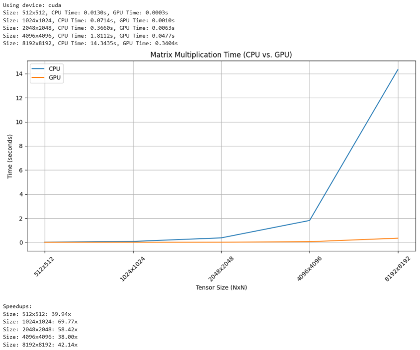
For a task such as matrix multiplication, fundamental to training neural networks, GPUs significantly accelerate the process compared to CPUs. However, financial AI is more than simply training models. It requires an end-to-end workflow that spans training, validation, deployment, and real-time inference.
In time-sensitive financial applications, GPUs minimize latency throughout the model lifecycle, from training and refinement to real-time execution.
- Training: Training deep learning models on massive datasets demands immense compute resources. GPUs accelerate the training process for complex neural network architectures by orders of magnitude, reducing development time and enabling faster experimentation
- Backtesting & validation: Backtesting is used to validate model performance under various historical market conditions. GPUs accelerate data replay simulations on historical data, enabling rapid iteration and optimization of model parameters. This accelerated feedback loop helps to test confidence in the model’s robustness before live deployment and allows for more extensive scenario analysis
- Deployment & inference: In live trading environments, models must generate predictions with near real-time speed. GPUs power real-time inference on streaming market data, ensuring trading decisions are executed as fast as possible
- Operationalization & model updates: Financial markets are dynamic, requiring continuous model adaptation. GPUs facilitate rapid model fine-tuning and retraining on new data, minimizing model drift and maximizing performance. The ability to integrate AI inference pipelines with q and PyKX ensures that models operate within the real-time data flow
Tools to fully leverage GPUs for deep learning
NVIDIA offers several tools to optimize and host deep learning models in production: Triton inference server, TensorRT, and NIMs.
- Triton inference server: Manages and serves deployed models for inference. Accessible within kdb+ over IPC. Triton allows for GPU acceleration of inferencing large models
- TensorRT: Optimizes deep learning models for GPU architecture, maximizing model throughput and minimizing latency for real-time inference
- NIMS: Provides the management layer, ensuring the health and performance of GPU infrastructure and the deployed models
These tools represent the software layer that optimizes deep learning models for GPUs and enables inferencing. This stack ties into kdb+ via a first-class function, allowing GPU inference within the kdb+ process directly upon the incoming data stream.
Finance use cases
| Pattern | Neural network(s) | Financial use cases |
| Anomaly detection |
|
|
| Classification |
|
|
| Clustering |
|
|
| Prediction forecasting |
|
|
| Reinforcement learning |
|
|
| Natural language processing (NLP) |
|
|
Key considerations:
- Data preprocessing: Financial data often requires extensive cleaning, transformation, and feature engineering before being ingested into a deep-learning model
- Model selection: The choice of neural network architecture depends on the specific problem and the characteristics of the data
- Hyperparameter tuning: Optimizing the hyperparameters of a deep learning model helps to achieve higher performance
- Overfitting: Deep learning models are prone to overfitting, especially with limited data, but techniques like regularization, dropout, and early stopping can help mitigate
- Explainability: Understanding why a deep learning model makes a particular prediction can be challenging
- Computational resources: Training deep learning models on large financial datasets requires significant computational resource
Training a model with kdb+
To demonstrate a deep learning framework, we will train and test an anomaly detection autoencoder to identify anomalous market data fluctuations caused by COVID-19.
Note that this simplified example is intended to show the overarching workflow; a real production use case would require more data and testing.
Method
The goal is to train a deep learning autoencoder using PyTorch that can identify anomalies in closing price and volume data from a kdb+ table. For simplicity, we will be training on cleaned daily data, but you could use hourly or even second data to improve this model. We will use AAPL close price and volume data from January 2016 to December 2019 to train our model and then test it on data from January 2020 through April 2020.
The code below walks through the steps for end-to-end experimentation; try it out yourself in Google Colab. You will also need to activate a free personal use license of PyKX.
Load data:
train_AAPL = kx.q(‘select from train_AAPL’) 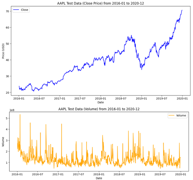
Configure training data:
train_table = train_AAPL[["Close", "Volume"]].reset_index()

# Get minimums and maximums to normalized the test data, MinMax scalar

close_min = train_table['Close'].min()
close_max = train_table['Close'].max()
volume_min = train_table['Volume'].min()
volume_max = train_table['Volume'].max()


# Normalize the data

train_table['Close'] = (train_table['Close'] - close_min) / (close_max - close_min)
train_table['Volume'] = (train_table['Volume'] - volume_min) / (volume_max - volume_min)


# Transform and format the PyKX table into a tensor

X_train_t = kx.q.flip(train_table._values).pt().type(torch.float32)


# Load tensor to GPU, if available

device = torch.device("cuda" if torch.cuda.is_available() else "cpu")
X_train_t = X_train_t.to(device)
train_dataset = TensorDataset(X_train_t, X_train_t)  # autoencoder => input=output
train_loader = DataLoader(train_dataset, batch_size=32, shuffle=True)
Define autoencoder and train model:
class Autoencoder(nn.Module):

    def __init__(self, input_dim=2, latent_dim=4):
        super(Autoencoder, self).__init__()


        # Encoder

        self.encoder = nn.Sequential(
            nn.Linear(input_dim, 8),
            nn.ReLU(),
            nn.Linear(8, latent_dim)
        )


        # Decoder

        self.decoder = nn.Sequential(
            nn.Linear(latent_dim, 8),
            nn.ReLU(),
            nn.Linear(8, input_dim)
        )

    def forward(self, x):
        z = self.encoder(x)
        out = self.decoder(z)
        return out

# Train the model and plot the loss

model = Autoencoder(input_dim=2, latent_dim=2).to(device)
criterion = nn.MSELoss()  # typical for reconstruction
optimizer = torch.optim.Adam(model.parameters(), lr=1e-3)
num_epochs = 30
train_losses = []

for epoch in range(num_epochs):
    epoch_loss = 0.0
    for batch_in, batch_out in train_loader:
        batch_in = batch_in.to(device)
        batch_out = batch_out.to(device)
        optimizer.zero_grad()
        output = model(batch_in)
        loss = criterion(output, batch_out)
        loss.backward()
        optimizer.step()
        epoch_loss += loss.item()
    avg_epoch_loss = epoch_loss / len(train_loader)
    train_losses.append(avg_epoch_loss)
    if (epoch+1) % 10 == 0:
print(f"Epoch [{epoch+1}/{num_epochs}] | Loss: {avg_epoch_loss:.6f}") 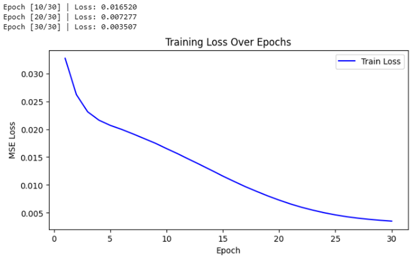
Load testing data:
# data frame used for evaluation
test_df = test_AAPL[[“Close”, “Volume”]].copy()

# PyKX table
test_AAPL = kx.q(‘select from test_AAPL’) 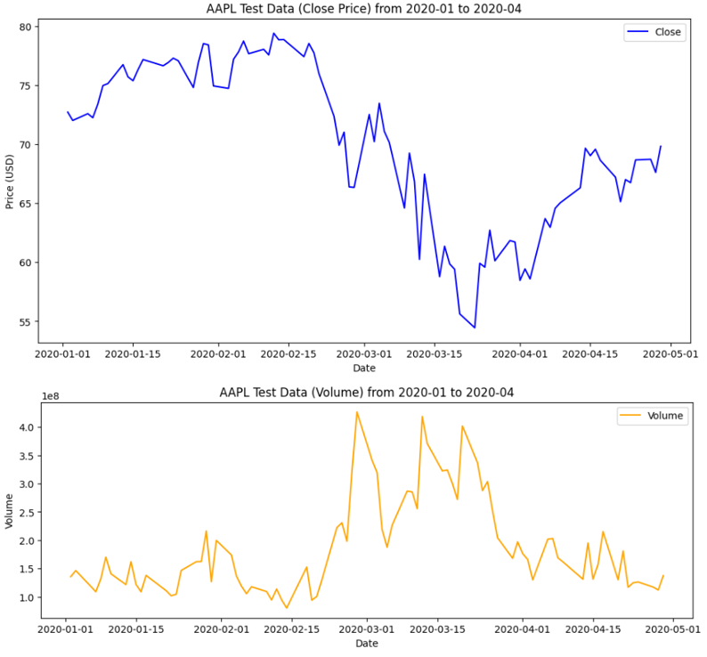
Test the autoencoder:
test_table = test_AAPL[["Close", "Volume"]].reset_index()

# Functions to standardize the test data, MinMax scalar
def Scalar_Price(x):
    minimum = test_table['Close'].min()
    maximum = test_table['Close'].max()
    return ((x-minimum)/(maximum-minimum))

def Scalar_Volume(x):
    minimum = test_table['Volume'].min()
    maximum = test_table['Volume'].max()
    return ((x-minimum)/(maximum-minimum))


# Standardize the data
test_table['Close'] = test_table['Close'].apply(Scalar_Price)
test_table['Volume'] = test_table['Volume'].apply(Scalar_Volume)


# To prepare our testing tensor, we remove the index 'Date' column
X_test_t = kx.q.qsql.delete(test_table, 'Date')


# Format and create the tensor
X_test_t = kx.q.flip(X_test_t._values).pt().type(torch.float32)


# Load the tensor to the device
X_test_t = X_test_t.to(device)
Model evaluation:
model.eval()
with torch.no_grad():
    recon_test = model(X_test_t)
    errors = torch.mean((recon_test - X_test_t) ** 2, dim=1)
errors_np = errors.cpu().numpy()
test_df["ReconstructionError"] = errors_np


# Example threshold from training distribution
X_train_t = X_train_t.to(device)
with torch.no_grad():
    recon_train = model(X_train_t)
    train_errors = torch.mean((recon_train - X_train_t) ** 2, dim=1)
train_errors_np = train_errors.cpu().numpy()
threshold = np.percentile(train_errors_np, 99)
test_df["Anomaly"] = test_df["ReconstructionError"] > threshold

print(test_df[30:60])
print(f"Number of anomalies in test set: {test_df['Anomaly'].sum()}")

>>> Number of anomalies in test set: 13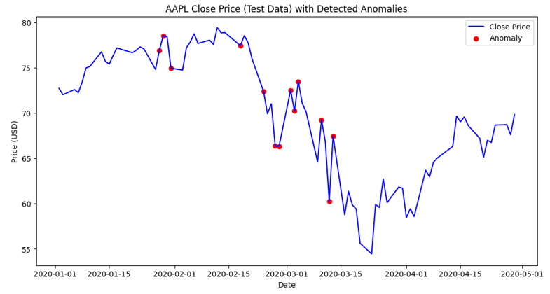
Outcome: We can see that that model successfully identified anomalous activity on and after February 20th, 2020.
Model validation and backtesting
After training a model, we need to test and validate unseen data. Successful validation confirms the model’s reliability for trading strategies. Then, the deep learning enhanced trading strategy can be backtested against historical market data to simulate real-world performance, assessing its effectiveness, risk factors, and potential profitability under past market conditions.
| Backtesting | Validation | |
| Definition | Testing on historical data to see how it would have performed | Checking how well a model generalizes to unseen data |
| Purpose | Evaluate the profitability, risk, and performance of a trading strategy | Assess model accuracy, robustness, and predictive power |
| Data used | Historical data (e.g., stock prices, indicators) | A separate data set not used in training |
| Focus | Simulating real-world trading conditions | Avoiding overfitting and ensuring generalization |
| Key metrics |
|
|
| Common in | Trading strategy development | Machine learning and AI-based financial models |
Validation involves evaluating the model’s performance on a separate validation dataset to fine-tune hyperparameters and detect overfitting. Common validation techniques include train-validation-test splits, k-fold cross-validation, and early stopping based on validation loss. Metrics such as mean squared error (MSE) for regression or accuracy, precision, recall, and F1-score for classification help assess model effectiveness. A well-validated deep learning model maintains a balance between bias and variance, preventing it from memorizing training data while ensuring it performs well in real-world scenarios.
Backtesting: Backtesting financial models is computationally demanding and time-consuming, requiring access to massive historical datasets often spanning years of market activity. It typically involves the following steps:
- Data replay: kdb+ enables rapid replay of historical market data. Analysts can simulate trading scenarios by feeding historical data to their trained models as if it were live data. This allows them to evaluate how the model would have performed in the past
- Performance evaluation: As the model processes the historical data, its predictions and trading decisions are recorded. Key performance metrics, such as returns, risk measures (e.g., sharpe ratio, maximum drawdown), transaction costs, and slippage, are calculated and analyzed
- Scenario analysis: kdb+ allows for flexible querying and filtering of historical data for scenario analysis. This involves testing the model’s performance under specific market conditions, such as periods of high volatility, market crashes, or economic events, to identify potential weaknesses in the model and assess its robustness
- Parameter optimization: Analysts can adjust the model’s parameters and retrain based on the backtesting results
Validation and testing are key steps in preparing a deep learning model for deployment and inference, ensuring that the model is reliable and resilient to the dynamic nature of the financial markets.
What’s next?
So far, we have learned about deep learning in financial markets, the required technologies, model training, validation, and backtesting. In the articles that follow, we will explore real-time inference, RAG-enhanced AI pipelines, visualization, and operationalization strategies.
Learn More
- Demystifying AI deployment: The role of Triton, TensorRT, and NIMS in everyday tech
- NVIDIA / KX blueprints
- kdb+ / q GPU Integration
- PyTorch
- Backtesting strategies in finance
- Backtesting at scale with highly performant data analytics
- Automated machine learning in kdb+
- Machine learning with kdb+
- Real-time machine learning to create stock predictions
You can also begin your journey with kdb+ by downloading our personal edition, or via one of our many courses on the KX Academy.