

Quantitative traders often use pattern matching in financial institutions to forecast market trends and enhance trading tactics. By detecting shapes, using methods such as head and shoulders or double bottoms, traders can predict when to buy or sell and increase profits based on historical price data.
These methods, however, can be slow and laborious, especially when dealing with millions of data points. With temporal similarity search (TSS), an integrated algorithm within KDB.AI, quants can now detect patterns efficiently and at scale without complex machine learning algorithms.
Let me show you how it works.
First, we will generate and normalize 10 million synthetic random walk data points.
n_points = 10_000_000
np.random.seed(42)  # Set seed for reproducibility

steps = np.random.choice([-1, 1], size=n_points)
random_walk = np.cumsum(steps)
normalized_walk = (random_walk - np.min(random_walk)) / (np.max(random_walk) - np.min(random_walk))
start_time = pd.Timestamp('2024-01-01 09:30:00')
time_series = pd.date_range(start=start_time, periods=n_points, freq='S')
synthetic_data = pd.DataFrame({
    'timestamp': time_series,
    'close': normalized_walk
})
Financial markets use the concept of random walks to model asset prices, suggesting that price changes are random and unpredictable. This aligns with the Efficient Market Hypothesis, which states that all known information is already reflected in prices.
Let’s plot our results into a graph.
plt.figure(figsize=(10, 5))
plt.plot(synthetic_data['timestamp'], synthetic_data['close'], linewidth=0.5)
plt.title('Normalized Random Walk (10 Million Data Points)')
plt.xlabel('Timestamp')
plt.ylabel('Normalized Close Price')
plt.show()
Now that our market data has been generated, we will initiate a session in KDB.AI.
If you want to follow along, visit https://trykdb.kx.com/.
KDBAI_ENDPOINT = (
    os.environ["KDBAI_ENDPOINT"]
    if "KDBAI_ENDPOINT" in os.environ
    else input("KDB.AI endpoint: ")
)
KDBAI_API_KEY = (
    os.environ["KDBAI_API_KEY"]
    if "KDBAI_API_KEY" in os.environ
    else getpass("KDB.AI API key: ")
)

session = kdbai.Session(api_key=KDBAI_API_KEY, endpoint=KDBAI_ENDPOINT)
With the session initiated, we will define our table, specifying the type: transformed similarity search and the metric Euclidean distance.
schema = {
    'columns': [
        {
            'name': 'timestamp',
            'pytype': 'datetime64[ns]'
        },
        dict(
            name='close',
            pytype='float64',
            vectorIndex=
                dict(
                    type='tss',
                    metric='L2'
                    )
            )
    ]
}
In the context of random walks, Euclidean distance analyzes how far the walk has deviated from a starting point or between any two points, providing insights into variability and spread over time.
Next, we will create the table and insert our synthetic market data.
# get the database connection. Default database name is 'default'
database = session.database('default')

# First ensure the table does not already exist
try:
    database.table("synthetic_data").drop()
    time.sleep(5)
except kdbai.KDBAIException:
    pass

# Create the table
table = database.create_table("synthetic_data", schema)

# Insert synthetic data
for i in range(0, len(synthetic_data), 600000):
    table.insert(synthetic_data.iloc[i:i+600000]) # get the database connection. Default database name is 'default'
database = session.database('default')

# First ensure the table does not already exist
try:
database.table("synthetic_data").drop()
time.sleep(5)
except kdbai.KDBAIException:
pass

# Create the table
table = database.create_table("synthetic_data", schema)

# Insert synthetic data
for i in range(0, len(synthetic_data), 600000):
table.insert(synthetic_data.iloc[i:i+600000])
Defining technical analysis patterns
Now that our table has been defined and our data ingested, we will create our functions. In this instance, and since our data has already been normalized, we will define these values as 0 and 1.
def create_pattern(pattern_type, length=100):
    if pattern_type == 'head_and_shoulders':
        points_x = np.array([0, 0.1, 0.25, 0.5, 0.75, 0.9, 1]) * length
        points_y = np.array([0.8, 1, 0.9, 1.2, 0.9, 1, 0.8])
        full_x = np.linspace(0, length, length)
        full_y = np.interp(full_x, points_x, points_y)
        return full_y
    elif pattern_type == 'cup_and_handle':
        x_cup = np.linspace(0, np.pi, int(0.8 * length))
        cup = np.sin(x_cup) * 0.5 + 0.5
        x_handle = np.linspace(0, 1, int(0.2 * length))
        handle = np.linspace(cup[-1], cup[-1] - 0.2, int(0.1 * length))
        handle = np.concatenate([handle, np.linspace(handle[-1], handle[0], int(0.1 * length))])
        return np.concatenate([cup, handle])
    elif pattern_type == 'uptrend':
        x = np.linspace(0, 1, length)
        return 0.8 * x + 0.2 * np.sin(10 * np.pi * x) + 0.5
    elif pattern_type == 'downtrend':
        x = np.linspace(0, 1, length)
        return -0.8 * x + 0.2 * np.sin(10 * np.pi * x) + 1
    elif pattern_type == 'double_bottom':
        x = np.linspace(0, 1, length)
        return 0.5 - 0.3 * np.abs(np.sin(2 * np.pi * x)) + 0.2
    else:
        raise ValueError("Invalid pattern type")

patterns = {
    'uptrend': create_pattern('uptrend'),
    'downtrend': create_pattern('downtrend'),
    'double_bottom': create_pattern('double_bottom'),
    'cup_and_handle': create_pattern('cup_and_handle'),
    'head_and_shoulders': create_pattern('head_and_shoulders'),
}
Analyzing with temporal similarity search
We will now use temporal similarity search to identify patterns in our market data.
Temporal similarity search (TSS) provides a comprehensive suite of tools for analyzing patterns, trends, and anomalies within time series datasets. TSS consists of two key components: transformed TSS and non-transformed TSS.
Transformed TSS specializes in highly efficient vector searches across massive time series datasets such as historical or reference data. Non-transformed TSS, which we will use in this example, is optimized for near real-time similarity search on fast-moving time series data.
Non-transformed TSS offers a dynamic method to search by giving the user the ability to change the number of points to match on runtime. Not only can this return the top-n most similar vectors, but it can also return the bottom-n or most dissimilar vectors. Perfect for use cases where understanding outliers and anomalies is paramount.
# Perform similarity search for each pattern and plot results
fig, axs = plt.subplots(len(patterns), 2, figsize=(15, 5*len(patterns)))

for i, (pattern_name, pattern_data) in enumerate(patterns.items()):
    # Normalize the pattern data
    pattern_data = (pattern_data - np.min(pattern_data)) / (np.max(pattern_data) - np.min(pattern_data))

    # Search for similar vectors in synthetic data
    nn_result = table.search([pattern_data.tolist()], n=1)[0]

    # Plot synthetic pattern
    axs[i, 0].plot(pattern_data)
    axs[i, 0].set_title(f'Synthetic {pattern_name.replace("_", " ").title()} Pattern')

    # Plot most similar synthetic pattern
    similar_pattern = nn_result.iloc[0]
    print(f"\nMost Similar Synthetic Pattern (at {similar_pattern['timestamp']}):")
    print(similar_pattern)

    # Try to find the matching pattern in the original synthetic data
    matching_index = synthetic_data[synthetic_data['timestamp'] == similar_pattern['timestamp']].index

    if not matching_index.empty:
        start_index = matching_index[0]
        end_index = start_index + 100

        if end_index > len(synthetic_data):
            end_index = len(synthetic_data)

        matching_data = synthetic_data.iloc[start_index:end_index]
        close_values_vector = matching_data['close'].tolist()

        print(close_values_vector)

        print("\nMatching data from original synthetic data:")
        print(matching_data)

        if not matching_data.empty:
            synthetic_pattern = matching_data['close'].values  # Ensure this is a NumPy array

            if len(synthetic_pattern) > 0:
                synthetic_pattern = (synthetic_pattern - np.min(synthetic_pattern)) / (np.max(synthetic_pattern) - np.min(synthetic_pattern))
                axs[i, 1].plot(synthetic_pattern)
                axs[i, 1].set_title(f'Most Similar Synthetic Pattern (at {similar_pattern["timestamp"]})')
            else:
                print("Error: Empty synthetic pattern")
        else:
            print("Error: No matching data found")
    else:
        print("No matching timestamp found.")

plt.tight_layout()
plt.show()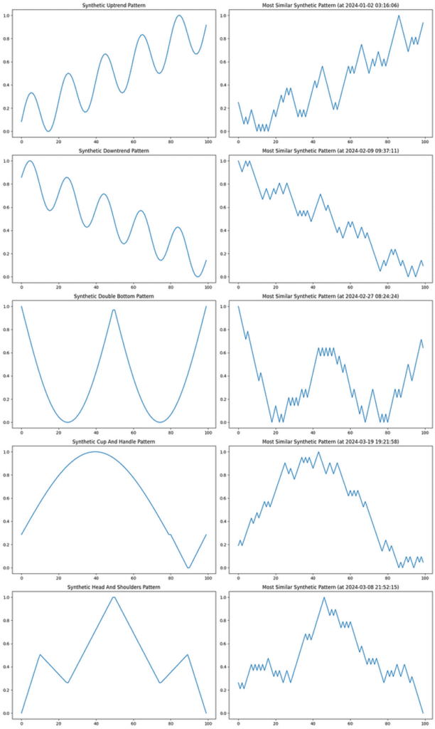
Why this matters
In our recent blog, Understand the heartbeat of Wall Street with temporal similarity search, we discussed how most banks have exceptional tick stores containing micro-movements of prices, trade executions, and related sentiment. With temporal similarity search, quantitative traders can identify similar patterns at scale, empowering them to:
- Quickly identify potential trading opportunities based on recognized patterns
- Backtest pattern-based trading strategies across extensive historical data
- Set up real-time alerts for when specific patterns emerge across multiple assets or markets
Of course, this isn’t just limited to financial applications; it could easily be deployed across other industries, including telecommunications, energy management, and transportation.
Read Turbocharge kdb+ databases with temporal similarity search, and check out our other articles at https://kdb.ai/learning-hub/ to learn more.
You can also discover other pattern and trend analysis use cases at kx.com.