
Processing and analyzing large financial datasets can be challenging, especially when dealing with Trade and Quote (TAQ) data, which provides quants and analysts with rich information regarding market activity. In this blog, I will demonstrate how kdb+, the world’s fastest analytical database, can mitigate these challenges and walk through common calculations such as VWAP and OHLC.
kdb+ offers several benefits for quants, from its small footprint and high-performant scalable architecture to the elegance and simplicity of its vector programming language q.
Let’s begin
Configure the environment
Step 1: Prerequisites
If you wish to follow along, you’ll need to download and install kdb+ on your machine. You can do so for free here.
Step 2: Download TAQ data
With our prerequisites met, we can now download a daily TAQ file from the NYSE. (Note: These files can be large, so downloading may take some time).
wget https://ftp.nyse.com/Historical%20Data%20Samples/DAILY%20TAQ/EQY_US_ALL_TRADE_20240702.gzStep 3: Clone the repository
Next, we will clone our kdb-taq repository, including the scripts and utilities required to process our data.
git clone https://github.com/KxSystems/kdb-taq.git
cd kdb-taq
This repository contains a script (tq.q) that helps process and load the data.
Step 4: Data preparation
With the repository cloned, we will now decompress our TAQ data and organize it into a usable directory for kdb+.
mkdir SRC
mv /path/to/EQY_US_ALL_TRADE_20240702.gz SRC/
gzip -d SRC/*
Step 5: Process the data
We will now use the tq.q script from the repository to process the raw TAQ data. We will also use the flags -s to specify the number of processing threads and SRC to define the file directory.
q tq.q -s 8 SRCProcessing will read and parse the raw data into a format suitable for querying.
Step 5: Load data into kdb+
Loading data into kdb+ is done using the \l command:
q)\l tqQuery the data
Now that our data has been successfully ingested into kdb+, we can run a few simple queries. Let’s begin by viewing the schema and structure of our trade table.
We will use the meta command to return column names and data types.
q)meta trade

c                                 | t f a
----------------------------------| -----
date                              | d
Time                              | n
Exchange                          | c
Symbol                            | s   p
SaleCondition                     | s
TradeVolume                       | i
TradePrice                        | e
TradeStopStockIndicator           | b
TradeCorrectionIndicator          | h
SequenceNumber                    | i
TradeId                           | C
SourceofTrade                     | c
TradeReportingFacility            | b
ParticipantTimestamp              | n
TradeReportingFacilityTRFTimestamp| n
TradeThroughExemptIndicator       | b
Example: Count the number of trades by stock
In our first example, we will explore the number of trades executed against each symbol and return the highest price.
q)select numTrade:count i, maxPrice:max TradePrice by Symbol from trade

Symbol | numTrade maxPrice
-------| -----------------
A      | 29655    133.03
AA     | 36623    41.15
AAA    | 51       25.07
AAAU   | 2786     23.13
AACG   | 108      0.86
AACI   | 6        11.45
AACT   | 1033     11.38
AACT.U | 1        10.745
AACT.WS| 24       0.1365
....
Query structures can affect performance. We can, however, use the function \t before our q expression to retrieve query duration.
q)\t select numTrade:count i, maxPrice:max TradePrice by Symbol from trade

113
Advanced analysis
Now that we understand how to load and query our TAQ data let’s explore more advanced calculations.
Example: Volume profile
Volume profiling helps traders understand the concentration of trades at various price levels throughout the day. By doing so, they can ascertain volume over time and make more informed decisions on entry and exit markers.
Using xbar, we can group the size of orders into 5-minute intervals:
q)select sum TradeVolume by 5 xbar time.minute from trade where symbol = `AAPL

minute| TradeVolume
------| -----------
04:00 | 10805
04:05 | 2257
04:10 | 1078
04:15 | 2216
04:20 | 1365
04:25 | 4717
...
We can also highlight the rolling sums for a symbol throughout the day.
q)select time, sums TradeVolume from trade where symbol = `AAPL

Time                 TradeVolume
--------------------------------
0D04:00:00.017646926 1
0D04:00:00.020101346 21
0D04:00:00.022979538 22
0D04:00:00.022987522 42
0D04:00:00.023776991 67
0D04:00:00.023920135 69
....
We can also visualize these events using tools such as KX Analyst or KX Developer (available for free).
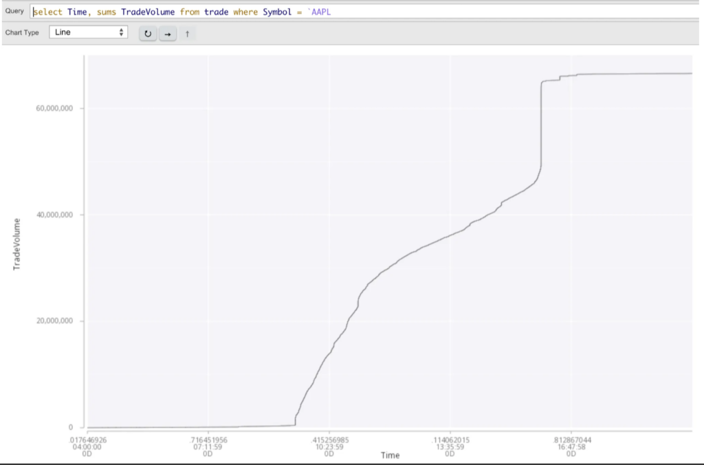
As you can see, the steep increases in the curve highlight periods of significant trading activity, reflecting market volatility or a heightened interest in a particular symbol. This is also helpful for analyzing intraday trends and periods of concentrated trading volume.
Example: Volume-weighted average
Volume-weighted averages reflect price movement more accurately by incorporating trading volume at different price levels. This is particularly useful in scenarios where traders wish to understand if movement is supported by strong market participation or a few solitary trades.
Let’s calculate the weighted average over time intervals using the function wavg.
q)select TradeVolume wavg TradePrice by Symbol from trade

Symbol | TradePrice
-------| ----------
A      | 126.0225
AA     | 40.73105
AAA    | 25.03718
AAAU   | 23.01037
AACG   | 0.8178756
AACI   | 11.37241
...
We can also query the weighted average over different time intervals.
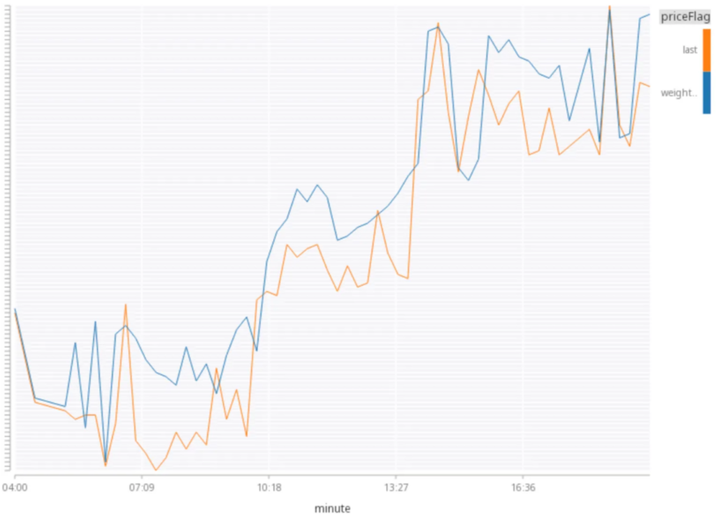
q)select LastPrice:last TradePrice,
         WeightedPrice:TradeVolume wavg TradePrice
   by 15 xbar Time.minute
   from trade
   where Symbol = `IBM

minute| LastPrice WeightedPrice
------| -----------------------
04:00 | 175.02    175.02
04:30 | 174.99    174.99
05:15 | 174.98    174.98
05:30 | 174.93    174.8051
05:45 | 174.96    174.91
06:00 | 174.96    174.9558
...
In this instance, we can see IBM’s daily price movements, with the “LastPrice” and “WeightedPrice” remaining closely aligned.
This indicates stable pricing with minimal influence from the trade volume, suggesting a moderate upward trend and positive market sentiment for IBM’s stock price.
Example: Open-high-low-close
Analysts often use methods such as OHLC to track securities’ short-term trends. Let’s create a simple query that calculates OHLC for a particular date, sym, and vwap over each 5-minute interval.
q)select low:min TradePrice,
         open:first TradePrice,
         close:last TradePrice,
         high:max TradePrice,
         volume:sum TradeVolume,
         vwap:TradeVolume wavg TradePrice
   by 5 xbar Time.minute
   from trade where Symbol=`AAPL

minute| low      open     close    high     volume  vwap
------| ----------------------------------------------------
04:00 | 215.89   216.6    216.11   216.6    10805   216.2432
04:05 | 216.1    216.18   216.27   216.27   2257    216.151
04:10 | 216.2    216.28   216.35   216.35   1078    216.2547
04:15 | 216.28   216.3    216.39   216.46   2216    216.3775
04:20 | 216.24   216.38   216.26   216.42   1365    216.3638
04:25 | 216.21   216.28   216.4    216.43   4717    216.323
.....
We can also extract the query as a function, enabling analysts to retrieve the results for a particular stock.
q)ohlcLookup:{[symbol]
    select low:min TradePrice,
           open:first TradePrice,
           close:last TradePrice,
           high:max TradePrice,
           volume:sum TradeVolume,
           vwap:TradeVolume wavg TradePrice
        by 5 xbar Time.minute
        from trade where Symbol=symbol}

q)ohlcLookup[`MSFT]

minute| low      open     close    high     volume  vwap
------| ----------------------------------------------------
04:00 | 455.29   456.2    455.61   456.7    5742    455.8347
04:05 | 455.11   455.5    455.32   455.67   1352    455.4394
04:10 | 455.07   455.33   455.37   455.47   1879    455.238
...

q)ohlcLookup[`GOOG]
minute| low      open     close    high     volume vwap
------| ---------------------------------------------------
04:00 | 183.94   184.01   184.14   184.38   2315   184.0851
04:05 | 183.97   184.07   184.02   184.07   373    184.0005
04:10 | 184.06   184.06   184.1    184.23   239    184.1581
...
By leveraging kdb+’s high-performance architecture and the simplicity of its vector programming language, q, analysts can efficiently perform various calculations such as volume profiling, volume-weighted averages, and open-high-low-close (OHLC) analysis to gain meaningful insights from massive datasets quickly and effectively.
If you have any questions or would like to know more, why not join our Slack community or begin your certification journey with our free curriculum on the KX Academy