As the volume of time-series data continues to surge, organizations face the challenge of turning it into actionable insights. Temporal similarity search (TSS), a built-in algorithm of the KDB.AI vector database, enables developers to quickly understand patterns, trends, and anomalies in time-series data without complex algorithms and machine learning tactics.
This blog will explore how to build a near real-time pattern-matching sensor pipeline to uncover patterns, predict maintenance, and enhance quality control. We will use Transformed Temporal Similarity Search to reduce the dimensionality of time series windows by up to 99% whilst preserving our original data shape to facilitate highly efficient vector search across our large-scale temporal dataset.
Let’s begin
Prerequisites for temporal similarity search
To follow along, please sign up for a free trial of KDB.AI at https://trykdb.kx.com/kdbai/signup and retrieve your endpoint and API key.
Let’s begin by installing our dependencies and importing the necessary packages.
!pip install kdbai_client matplotlib
# read data
from zipfile import ZipFile
import pandas as pd

# plotting
import matplotlib.pyplot as plt

# vector DB
import os
import kdbai_client as kdbai
from getpass import getpass
import time
Data ingest and preparation
Once the prerequisites are complete, we can download and ingest our dataset. In this instance, we are using water pump sensor data from Kaggle, which contains raw data from 52 pump sensors.
# Download and unzip our time-series sensor dataset
def extract_zip(file_name):
    with ZipFile(file_name, "r") as zipf:
        zipf.extractall("data")

extract_zip("data/archive.zip")

# Read in our dataset as a Pandas DataFrame
raw_sensors_df = pd.read_csv("data/sensor.csv")
show_df(raw_sensors_df)
Raw IoT sensor data
# Drop duplicates
sensors_df = raw_sensors_df.drop_duplicates()

# Remove columns that are unnecessary/bad data
sensors_df = sensors_df.drop(["Unnamed: 0", "sensor_15", "sensor_50"], axis=1)

# convert timestamp to datetime format
sensors_df["timestamp"] = pd.to_datetime(sensors_df["timestamp"])

# Removes rows with any NaN values
sensors_df = sensors_df.dropna()

# Reset the index
sensors_df = sensors_df.reset_index(drop=True)
The dataframe contains a column named ‘machine_status’ with information on sensors with a ‘BROKEN’ status. Let’s plot and visualize a sensor named ‘Sensor_00’.
# Extract the readings from the BROKEN state of the pump
broken_sensors_df = sensors_df[sensors_df["machine_status"] == "BROKEN"]

# Plot time series for each sensor with BROKEN state marked with X in red color
plt.figure(figsize=(18, 3))
plt.plot(
    broken_sensors_df["timestamp"],
    broken_sensors_df["sensor_00"],
    linestyle="none",
    marker="X",
    color="red",
    markersize=12,
)
plt.plot(sensors_df["timestamp"], sensors_df["sensor_00"], color="blue")
plt.show()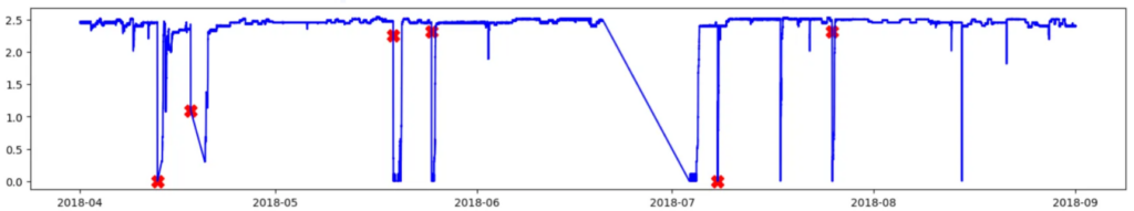
As you can see from the output, the blue line represents typical sensor parameters of approximately 2.5 but occasionally drops to between 0 – 0.5 due to sensor failure.
Let’s filter our dataframe for sensor_00 and group the values into time windows.
sensor0_df = sensors_df[["timestamp", "sensor_00"]]
sensor0_df = sensor0_df.reset_index(drop=True).reset_index()

# This is our sensor data to be ingested into KDB.AI
sensor0_df.head()
# Set the window size (number of rows in each window)
window_size = 100
step_size = 1

# define windows
windows = [
    sensor0_df.iloc[i : i + window_size]
    for i in range(0, len(sensor0_df) - window_size + 1, step_size)
]

# Iterate through the windows & extract column values
start_times = [w["timestamp"].iloc[0] for w in windows]
end_times = [w["timestamp"].iloc[-1] for w in windows]
sensor0_values = [w["sensor_00"].tolist() for w in windows]

# Create a new DataFrame from the collected data
embedding_df = pd.DataFrame(
    {"timestamp": start_times, "sensor_00": sensor0_values}
)

embedding_df = embedding_df.reset_index(drop=True).reset_index()

embedding_df.head()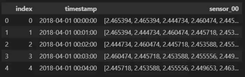
Store and manage in KDB.AI
As shown above, each data point has a 100-dimension time window (column ‘sensor_00’) representing the value at the timestamp and the previous 99 entries.
Let’s store these values in KDB.AI and perform a similarity search.
We will begin by defining our endpoint and API key.
KDBAI_ENDPOINT = (
    os.environ["KDBAI_ENDPOINT"]
    if "KDBAI_ENDPOINT" in os.environ
    else input("KDB.AI endpoint: ")
)
KDBAI_API_KEY = (
    os.environ["KDBAI_API_KEY"]
    if "KDBAI_API_KEY" in os.environ
    else getpass("KDB.AI API key: ")
)

session = kdbai.Session(api_key=KDBAI_API_KEY, endpoint=KDBAI_ENDPOINT)
Once connected, we will define our schema, table, indexes, and embedding configuration.
# get the database connection. Default database name is 'default'
database = session.database('default')

# Set up the schema and indexes for KDB.AI table, specifying embeddings column with 384 dimensions, Euclidean Distance, and flat index
sensor_schema = [
    {"name": "index", "type": "int64"},
    {"name": "timestamp", "type": "datetime64[ns]"},
    {"name": "sensor_00", "type": "float64s"}
]

indexes = [
    {
        "name": "flat_index",
        "type": "flat",
        "column": "sensor_00",
        "params": {"metric": "L2"},
    }
]

embedding_conf = {'sensor_00': {"dims": 8, "type": "tsc", "on_insert_error": "reject_all" }}
What have we just done:
- The schema defines the following columns to be used in the table
- index: Unique identifier for each time series window
- timestamp: The first value in the time series window for that row/index
- sensor_00: Where time series windows will be stored for TSS
- Indexes
- name: User-defined name of index
- type: (Flat index, qFlat(on-disk flat index), HNSW, qHNSW, IVF, orIVFPQ)
- column: the column index applies: In this instance, ‘sensor_00’
- params: Search metric definition (L2-Euclidean Distance)
- embedding_conf: Configuration information for search
- dims=8: compressing the 100-dimension incoming windows into eight dimensions for faster, memory-efficient similarity search!
- type: ‘tsc’ for transformed temporal similarity search.
Learn more by visiting KDB.AI learning hub articles
Let’s now create our table using the above settings.
# First ensure the table does not already exist
try:
    database.table("sensors").drop()
    time.sleep(5)
except kdbai.KDBAIException:
    pass


# Create the table called "sensors"
table = database.create_table("sensors",
                              schema = sensor_schema,
                              indexes = indexes,
                              embedding_configurations = embedding_conf)

# Insert our data into KDB.AI
from tqdm import tqdm
n = 1000  # number of rows per batch

for i in tqdm(range(0, embedding_df.shape[0], n)):
    table.insert(embedding_df[i:i+n].reset_index(drop=True))
Identify failures using temporal similarity search
We will now look to identify all failures in our table by identifying the first failure and then using its associated time window as a query vector.
broken_sensors_df["timestamp"] Notice the first broken index at 17,125. To capture the moments before the failure, we will define our query vector as 17,100.
# This is our query vector, using the 17100th window as an example
# (this is just before the first instance when the sensor is in a failed state)
q = embedding_df['sensor_00'][17100]

# Visualise the query pattern
plt.figure(figsize=(10, 6))
plt.plot(embedding_df['sensor_00'][17100], marker="o", linestyle="-")
plt.xlabel("Timestamp")
plt.ylabel("Value")
plt.title("Query Vector")
plt.grid(True)
plt.xticks(rotation=45)  # Rotate x-axis labels for readability
plt.show()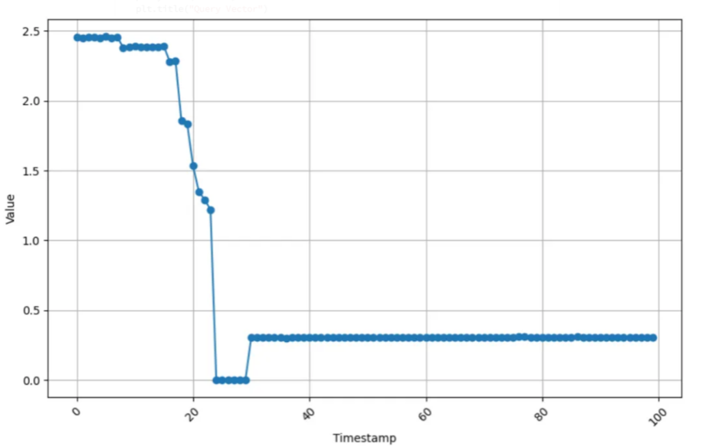
Now, we will execute a search to find the top 100 matches of potential sensor failure.
nn1_result = table.search(vectors={'flat_index': [q]}, n=100, filter=[(">","index", 18000)])
nn1_result[0]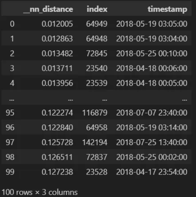
Notice that the first matches are indexed as 64,949 and 64,948, suggesting overlap due to our 100-dimension window. We can alleviate this with a filter.
def filter_results(df, range_size=200):

    final_results = []
    removed_indices = set()

    for _, row in df.iterrows():
        current_index = row['index']

        # If this index hasn't been removed
        if current_index not in removed_indices:
            final_results.append(row)

            # Mark indices within range for removal
            lower_bound = max(0, current_index - range_size // 2)
            upper_bound = current_index + range_size // 2
            removed_indices.update(range(lower_bound, upper_bound + 1))

    # Create a new dataframe from the final results
    final_df = pd.DataFrame(final_results)

    return final_df

filtered_df = filter_results(nn1_result[0])

# Display the filtered results
print(filtered_df)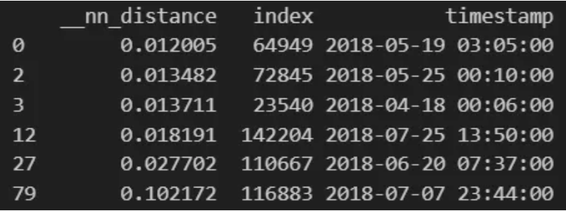
Once filtered, we can easily identify pattern similarities and predict when failure has occurred.
Let’s compare it against our original data.
broken_sensors_df["timestamp"]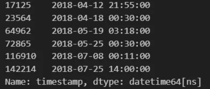
Notice the comparison in our results, capturing each failed state timestamp within a few indexes. We can also see an anomaly, which could indicate a potential missed failed state.
Finally, we will visualize our results.
for i in filtered_df['index']:
    plt.plot(embedding_df['sensor_00'][i], marker="o", linestyle="-")

plt.xlabel("Timestamp")
plt.ylabel("Value")
plt.title("Query & Similar Patterns")
plt.grid(True)
plt.xticks(rotation=45)  # Rotate x-axis labels for readability
plt.show()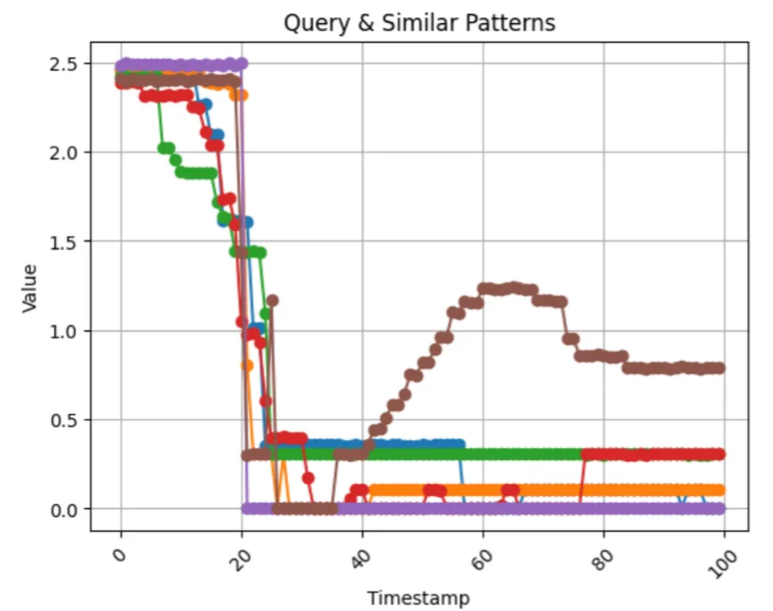
In this blog, I have demonstrated how transformed TSS can help identify instances of IoT failure in temporal datasets without implementing complex statistical methods or machine learning.
To learn more about this process, check out our documentation and samples on the KDB.AI learning hub. You can also download the notebook from our GitHub repository or open it directly in Google Colab.