

Co-author: Ryan Siegler
In my previous article, GPU-accelerated deep learning with kdb+, we explored training, validating, and backtesting a deep-learning model for algorithmic trading in financial markets. In this article, we will explore the next challenge, high-speed inference, and how integrating GPU-accelerated models directly within your kdb+ data processes can help streamline analytics directly on data, reduce latency, and harness the value of real-time decision-making.
While model training is often the key focus in deep learning, the demands of high-velocity data, especially in financial markets, necessitate optimizing inference performance. GPU-accelerated models can process incoming data streams as they arrive, resulting in faster decision-making, optimized trading strategies, increased alpha, and mitigation of lost profits. A real-time inference system can also assist in model drift detection, which occurs when data ingested into a model statistically differs from its original training data. It also makes monitoring performance metrics (recall, precision, accuracy, etc.) on the newest data possible, detecting model drift quickly for recalibration and fine-tuning.
The inference stack
The following technologies will enable and accelerate real-time inference in our deep-learning models:
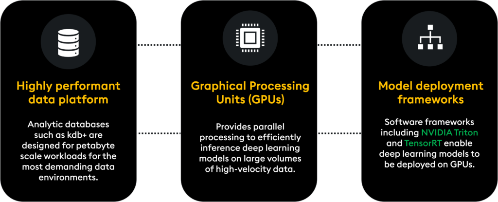
High-performance data platform:
- Databases such as kdb+ can ingest and process petabyte-scale data streams for deep learning models and process results for trading decisions
Model deployment frameworks: Inference models on GPU infrastructure:
- GPUs provide the parallel processing power needed to efficiently inference deep learning models on large volumes of high-velocity data
- Software frameworks like NVIDIA’s Triton and TensorRT enable deep learning models to deploy on GPU infrastructures
Let’s take a closer look at these components.
High-performance data platform:
kdb+ excels at low-latency capturing and processing high-frequency data, a feature necessary for real-time inference. By merging deep learning models into kdb+ processes, you streamline data handling and reduce the time from data arrival to predictive insights.
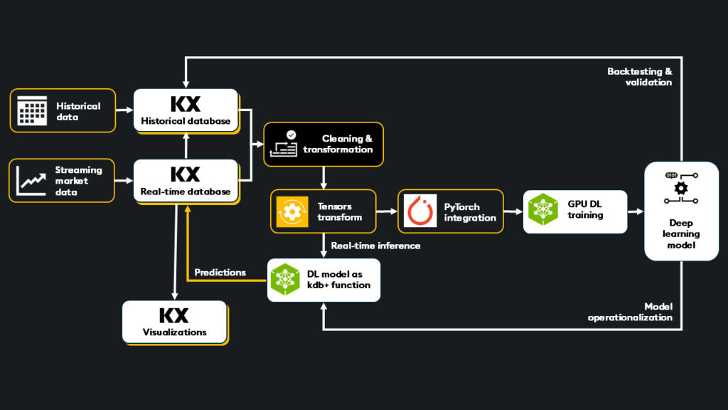
Real-time data for inference: kdb’s real-time tick architecture, designed for time-series data, is an all-in-one platform for capturing real-time data streams. It ensures new data is cleaned, transformed, and presented to the deep learning model, reducing unnecessary round trips to external systems.
Model-to-data architecture: Within the kdb+ real-time tick architecture, your model will directly subscribe to live data flows as a first-class function, embedding your model into your data. This provides minimal latency and minimizes the need to transfer large amounts of data between systems.
Data transformation & filtering: kdb+’s powerful q language and pythonic interface PyKX can efficiently prepare data for deep learning models. By performing lightning-fast cleaning, transformation, aggregation, filtering, and tensor generation, it ensures that only high-quality, relevant data is passed to the model for inference.
Predictive outputs combined directly with existing data: With your model embedded into your data via kdb+, predictive outputs can be joined directly into existing data tables. This allows developers to design custom logic and additional aggregations to perform further analysis, run advanced queries, or trigger trading actions.
GPU integration: kdb+ integrates with GPU inferencing services like NVIDIA Triton and TensorRT, leveraging the power of GPUs for ultra-low latency inference on streaming market data.
Integration with deep learning frameworks: PyKX offers tensor conversion to prepare data for inference and fine-tuning. Tensors are the fundamental data structure for deep learning frameworks like PyTorch.
Example (Try it in Colab)
os.environ['PYKX_BETA_FEATURES'] = 'True'
import pykx as kx
kx.q.til(10).pt()  # Converts kdb+ data to a PyTorch tensor
>>> tensor([0, 1, 2, 3, 4, 5, 6, 7, 8, 9])
Performance monitoring: With the most recent inference results available directly alongside existing data, monitoring accuracy with performance metrics (recall, precision, accuracy, etc.) can help to identify when a model has drifted and needs retraining quickly.
kdb+ empowers developers to build truly integrated, lightning-fast inference pipelines. Coupled with GPU acceleration and NVIDIA’s Triton inference server, deploying deep learning models for real-time inference and continuous learning will ensure competitive performance and actionable insights now, not later.
Model deployment frameworks: Inference models on GPU infrastructure
Deploying deep learning models on GPU infrastructure requires model-level optimization and efficient serving mechanisms for optimal inference. NVIDIA provides two key technologies: TensorRT, which optimizes models for peak performance, and Triton Inference Server, which manages large-scale, multi-model deployment with dynamic batching and orchestration.
TensorRT
NVIDIA TensorRT is a high-performance deep learning inference library that optimizes trained models for deployment on NVIDIA GPUs. Its primary purpose is to optimize models to accelerate inference, which makes it ideal for latency-sensitive and real-time applications.
Key features:
- Model optimization: TensorRT performs graph optimizations, such as layer fusion and kernel auto-tuning, to enhance execution efficiency. It also supports precision calibration, allowing models trained in FP32 to execute in FP16 or INT8, reducing memory usage and increasing throughput without significant accuracy loss
- Broad framework support: TensorRT integrates with popular deep learning frameworks like TensorFlow and PyTorch. Developers can import models in the ONNX format or utilize framework-specific parsers like torch_tensorrt, facilitating a smooth transition from training to deployment
- TensorRT inference engine: Create a TensorRT engine from your ONNX or framework-specific format model to inference accelerated models on GPU infrastructure
- Extensible architecture: For unique or unsupported operations, TensorRT allows the creation of custom layers through its plugin API. This extensibility ensures that specialized models can still benefit from TensorRT’s optimization capabilities
Example
import torch
import torch_tensorrt
import time

# 1. Define a CNN model

class ComplexCNN(torch.nn.Module):
    def __init__(self):
        super().__init__()
        self.conv1 = torch.nn.Conv2d(3, 64, kernel_size=3, padding=1)
        self.relu1 = torch.nn.ReLU()
        self.conv2 = torch.nn.Conv2d(64, 128, kernel_size=3, padding=1)
        self.relu2 = torch.nn.ReLU()
        self.pool1 = torch.nn.MaxPool2d(2, 2)
        self.conv3 = torch.nn.Conv2d(128, 256, kernel_size=3, padding=1)
        self.relu3 = torch.nn.ReLU()
        self.conv4 = torch.nn.Conv2d(256, 512, kernel_size=3, padding=1)
        self.relu4 = torch.nn.ReLU()
        self.pool2 = torch.nn.MaxPool2d(2, 2)
        self.fc1 = torch.nn.Linear(512 * 8 * 8, 1024)
        self.relu5 = torch.nn.ReLU()
        self.fc2 = torch.nn.Linear(1024, 10)

    def forward(self, x):
        x = self.pool1(self.relu2(self.conv2(self.relu1(self.conv1(x)))))
        x = self.pool2(self.relu4(self.conv4(self.relu3(self.conv3(x)))))
        x = x.view(x.size(0), -1)  # Flatten
        x = self.relu5(self.fc1(x))
        x = self.fc2(x)
        return x


# 2. Setup: Device, Model, Input

device = "cuda" if torch.cuda.is_available() else "cpu"
model = ComplexCNN().to(device)
input_shape = (1, 3, 32, 32)
dummy_input = torch.randn(input_shape).to(device)


# 3. Compile with Torch-TensorRT (using FP16 if available)

enabled_precisions = {torch.float32}
if torch.cuda.is_available() and torch.cuda.get_device_capability()[0] >= 7:  # Check for FP16 support
    enabled_precisions = {torch.float16}
    print("Using FP16 precision.")
else:
    print("Using FP32 precision.")

trt_model = torch_tensorrt.compile(
    model,
    inputs=[torch_tensorrt.Input(input_shape)],
    enabled_precisions=enabled_precisions,
)


# Function to measure speed

def measure_inference(model, input_data, num_iterations=1000, warmup_iterations=10):
    with torch.no_grad():
        for _ in range(warmup_iterations): #warmup iterations
            model(input_data)
        total_time = 0.0
        for _ in range(num_iterations):
            start_time = time.time()
            model(input_data)
            total_time += time.time() - start_time
    return num_iterations / total_time

input_data = torch.randn(input_shape).to(device)


# 4. Measure PyTorch Throughput (Inferences per second)

pytorch_throughput = measure_inference(model, input_data)
print(f"PyTorch Throughput: {pytorch_throughput:.2f} inferences/second")


# 5. Measure TensorRT Throughput (Inferences per second)

tensorrt_throughput = measure_inference(trt_model, input_data)
print(f"TensorRT Throughput: {tensorrt_throughput:.2f} inferences/second")


# 6. Print Throughput Speedup

speedup = tensorrt_throughput / pytorch_throughput
print(f"Throughput Speedup: {speedup:.2f}x")
Results:
- PyTorch Throughput: 1201.83 inferences/second
- TensorRT Throughput: 2820.98 inferences/second
- Throughput Speedup: 2.35x
NVIDIA Triton inference server
NVIDIA Triton inference server is an open-source software solution designed to streamline the deployment of deep learning models across diverse environments. While TensorRT focuses on single-model optimization, Triton focuses on system-level efficiency by ensuring high-performance and dynamically scaling inference on GPU and CPU infrastructures.
Key features:
- Framework agnosticism: Triton supports models from all major machine learning frameworks, including TensorFlow, PyTorch, ONNX, TensorRT, and more. This flexibility allows developers to deploy models without requiring extensive refactoring or conversion
- Dynamic batching and concurrent model execution: To optimize resource utilization and throughput, Triton offers dynamic batching capabilities, aggregating multiple inference requests to process them simultaneously. Additionally, it can run multiple models concurrently, efficiently managing hardware resources to meet varying application demands
- Scalability across deployment environments: Whether operating in cloud data centers, on-premises servers, or edge devices, Triton provides a consistent inference platform. It integrates seamlessly with orchestration tools like Kubernetes, facilitating scalable and resilient model deployments
- Comprehensive monitoring and metrics: Triton includes logging and monitoring features, offering real-time insights into model performance and system utilization. This transparency aids in fine-tuning models and infrastructure for optimal inference efficiency
Learn more about NVIDIA Triton, and see the triton-inference-server GitHub.
TensorRT and Triton serve distinct but complementary roles in GPU-accelerated inference pipelines. TensorRT optimizes individual models for peak performance, which is perfect for latency-sensitive applications like high-frequency trading. Triton deploys and manages models at scale, particularly useful for managing multiple models, dynamic batching, and integration with Kubernetes-based deployments.
Integrating GPU inference with kdb+
Once your model is optimized with TensorRT, it can be inferenced directly via TensorRT or using the Triton inference server. kdb+ can invoke inference from within a kdb+ function using inter-process communication (IPC) or API calls. The kdb+ process, with direct access to streamed data, passes relevant data to GPU-based inference engines, triggering predictions with minimal latency.
The benefit of stacking these technologies is ensuring that real-time data is served directly to GPU-powered inference. This means minimal data movement between systems and predictions combined directly back into the data pipeline for further insights.
End-to-end workflow
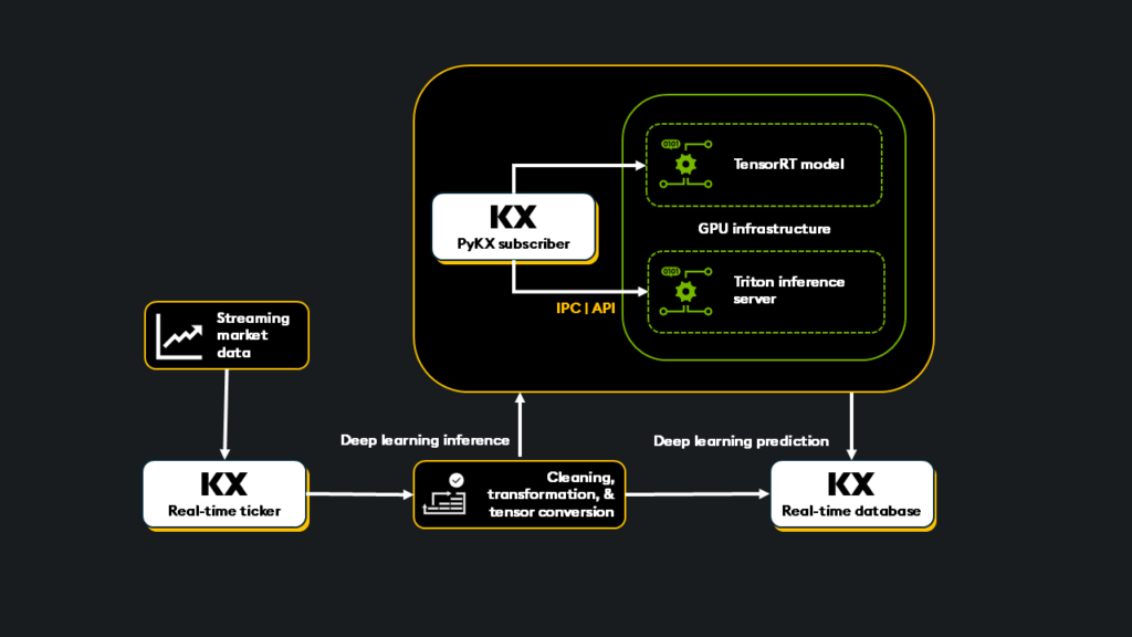
- Live market data is captured with kdb+/PyKX real-time tick architecture.
- Data is cleaned, transformed, and filtered for inference using PyKX or q.
- The TensorRT optimized model is wrapped in a kdb+ function or PyKX real-time subscriber and called for inference. NVIDIA Triton manages the inference of the TensorRT optimized model and is called by kdb+/PyKX via IPC or API.
- Inference results are written back as a new kdb+/PyKX column.
Example
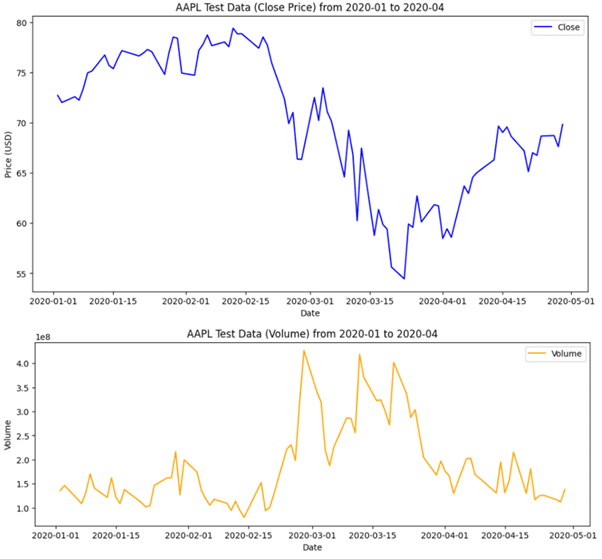
In the following example, we will construct an anomaly detection system to monitor AAPL (Apple) stock data. We will train an autoencoder, optimize it for GPU inference with TensorRT, and then deploy it with PyKX.
Step 1: Train an autoencoder anomaly detection model:
In my previous article – GPU accelerated deep learning with kdb+– I explored how to train this model. For continuity, I will reference the architecture below.
# The architecture of our autoencoder model:

import torch.nn as nn
import torch.nn.functional as F

class Autoencoder(nn.Module):
    def __init__(self, input_dim=2, latent_dim=4):
        super(Autoencoder, self).__init__()


        # Encoder

        self.encoder = nn.Sequential(
            nn.Linear(input_dim, 8),
            nn.ReLU(),
            nn.Linear(8, latent_dim)
        )


        # Decoder

        self.decoder = nn.Sequential(
            nn.Linear(latent_dim, 8),
            nn.ReLU(),
            nn.Linear(8, input_dim)
        )

    def forward(self, x):
        z = self.encoder(x)
        out = self.decoder(z)
        return out

model = Autoencoder(input_dim=2, latent_dim=4).to(device)
Step 2: Create a TensorRT model from PyTorch autoencoder model:
#Setup and Imports:

import yfinance as yf
import pandas as pd
import numpy as np
import torch
import torch_tensorrt
from torch.utils.data import TensorDataset, DataLoader
import matplotlib.pyplot as plt
import os
os.environ['PYKX_BETA_FEATURES'] = 'True'
import pykx as kx


# The shape of input data that that will be passed to the model during inference

input_shape = (1,2)
enabled_precisions = {torch.float32}

# Create the TensorRT model

trt_model = torch_tensorrt.compile(
    model,
    inputs=[torch_tensorrt.Input(input_shape)],
    enabled_precisions=enabled_precisions,
)


# Save the compiled TensorRT model

torch_tensorrt.save(trt_model, "trt_model.ts")
Step 3: Real-Time Inference:
Now that we’ve completed training and optimizing a TensorRT model for GPU-accelerated inference, we can deploy it within a real-time PyKX architecture.
To do so, we will use the following components and workflow.
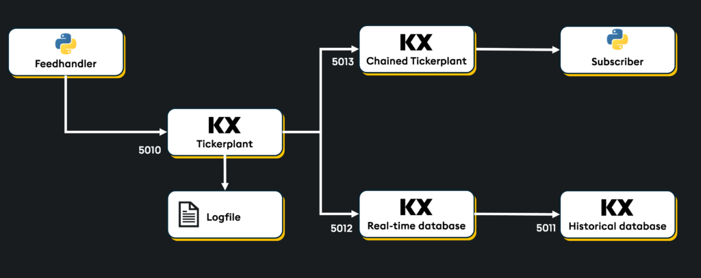
- Tickerplant: Publishes and logs live data stream to the real-time database (RDB) and other subscribed processes.
- Real-time database (RDB): Stores live data.
- Historical database (HDB): Stores historical data pushed daily from the real-time database (RDB).
- Chained Tickerplant: Subscribes to and receives live data from Tickerplant.
- Subscriber (real-time process): Subscribes to and receives live data from the chained tickerplant. This is where the GPU-optimized TensorRT model will be used for inference, determine data anomalies, and publish back to the RDB.
#Load Data for Inference
test_data = kx.q(‘select from test_AAPL’).
Step 4: Create a feed.py file to stream this AAPL data into your real-time architecture
%%writefile feed.py

# feed.py
import time
import yfinance as yf
import pykx as kx

test_data = yf.download(
    tickers="AAPL",
    start="2020-01-01",
    end="2020-4-30",
    interval="1d",
    auto_adjust=True
)
test_data.dropna(inplace=True)

# Create our PyKX table of test data
test_table = kx.toq(test_data.droplevel(level='Ticker', axis=1))
test_table = test_table[["Close","Volume"]].reset_index()

test_table['time'] = kx.TimespanAtom('now')
test_table['sym'] = 'AAPL'
new_order = ['time','sym', 'Date', 'Close', 'Volume']
test_table = test_table[new_order]

def main():
  with kx.SyncQConnection(port=5010, wait=True, no_ctx=True) as q:
    for row in kx.q.flip(test_table._values):
      formatted_row = [[val] for val in row]
      print(formatted_row)
      q('.u.upd', 'AAPL', formatted_row)
      print(f"Published: {row}")
      time.sleep(1)

if __name__ == '__main__':
    try:
        main()
    except KeyboardInterrupt:
        print('Data feed stopped')
Step 5: Define schemas for real-time architecture
Let’s define two tables in our real-time database (RDB), one named ‘AAPL’, to store incoming stock data and another named ‘AAPL_Anomaly’, to store data after it has been passed through the TensorRT anomaly detection model.
AAPL = kx.schema.builder({
    'time': kx.TimespanAtom,
    'sym': kx.SymbolAtom,
    'Date': kx.TimestampAtom,
    'Close': kx.FloatAtom,
    'Volume': kx.LongAtom,

})

AAPL_ANOMALY = kx.schema.builder({
    'time': kx.TimespanAtom,
    'sym': kx.SymbolAtom,
    'Date': kx.TimestampAtom,
    'Close': kx.FloatAtom,
    'Volume': kx.LongAtom,
    'Anomaly': kx.BooleanAtom,
})
Step 6: Build a tickerplant, RDB, and HDB
simple = kx.tick.BASIC(
    tables = {'AAPL': AAPL, 'AAPL_ANOMALY': AAPL_ANOMALY},
    ports={'tickerplant': 5010, 'rdb': 5012, 'hdb': 5011},
    log_directory = 'log',
    database = '.',
)
simple.start()
Step 7: Create a chained tickerplant & subscriber
Now let’s complete the architecture by adding a chained tickerplant and configure it to retrieve data from the main tickerplant. A subscriber will also be configured to pull live data from the chained tickerplant and inference via the TensorRT model.
# Create and start the chained Tickerplant
chained_tp = kx.tick.TICK(port=5013, chained=True, process_logs='tp.txt')
chained_tp.start({'tickerplant': 'localhost:5010'})

# Create the subscriber, a Real-time processor
rte = kx.tick.RTP(port=5014, subscriptions = ['AAPL'], vanilla=False, process_logs='rte.txt')

# Define a pre_processor and post_processor for the subscriber

# preprocessor checks that the AAPL table is present in the Tickerplant
def pre_processor(table, message):
    if table in ['AAPL']:
      return message
    return None

# Postprocessor normalizes, transforms live data into tensors, and inferences the TensorRT model upon this incoming live data.

def post_processor(table, message):
  import os
  import time
  import torch
  import torch_tensorrt

  os.environ['PYKX_BETA_FEATURES'] = 'True'
  test_table = message.select(columns = kx.Column('Close') & kx.Column('Volume'))

  # values for normalization from previous data
  close_min = 20
  close_max = 71
  volume_min = 45448000
  volume_max = 533478800
  # normalize the data
  test_table['Close'] = (test_table['Close'] - close_min) / (close_max - close_min)
  test_table['Volume'] = (test_table['Volume'] - volume_min) / (volume_max - volume_min)

  # Transform to tensors
  X_test_t = kx.q.flip(test_table._values).pt().type(torch.float32)

  # Load tensor to GPU, if available
  device = torch.device("cuda" if torch.cuda.is_available() else "cpu")
  X_train_t = X_test_t.to(device)

  # Load the saved trt_model (automatically uses available GPU)
  trt_model = torch_tensorrt.load("trt_model.ts").module()

  # Run new data through the TensorRT model
  with torch.no_grad():
      recon_test = trt_model(X_train_t)
      error = torch.mean((recon_test - X_train_t) ** 2, dim=1)
  print(error)

  # If error is above a certain threshold, it is an anomaly
  if error > 0.001:
    message['Anomaly'] = True
  else:
    message['Anomaly'] = False

  # Publish the message with the new 'Anomaly' column to the AAPL_ANOMALY table in the RDB
  with kx.SyncQConnection(port=5010, wait=True, no_ctx=True) as q:
      q('.u.upd', 'AAPL_ANOMALY', message._values)

  return None

# Set up and start the real time processor (subscriber)
rte.libraries({'kx': 'pykx'})
rte.pre_processor(pre_processor)
rte.post_processor(post_processor)
rte.start({'tickerplant': 'localhost:5013'})

# Start the live data feed
import subprocess
import sys
with kx.PyKXReimport():
    feed = subprocess.Popen(
        ['python', './feed.py'],
        stdin=subprocess.PIPE,
        stdout=None,
        stderr=None,
    )

Results: Now the data is flowing through our architecture, the TensorRT model is detecting anomalies on streamed data. Let’s take a look at the results in the ‘AAPL_ANOMALY’ table in the RDB:

simple.rdb('AAPL_ANOMALY')
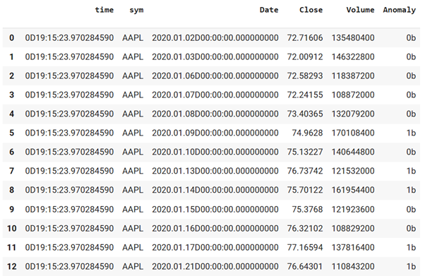
This end-to-end pipeline achieves high-performance, GPU-accelerated deep learning inference on streaming data. By seamlessly integrating predictions into RDB tables via PyKX, we can unlock immediate insights for data-driven decisions.
Combining predictions with data for further analytics and decisioning
Now that the model produces real-time predictions, what will you do with them? How can they be leveraged to drive deep insights and informed decisions within the same high-performance environment?
- Immediate post-processing: Merging and enriching data with predictions from inference ties deep learning results directly to your kdb+/PyKX tables. With these predictions now a part of your dataset, next-level analytics can be applied. This can include a variety of time-series analytics (including as-of joins), pattern matching, anomaly detection with Temporal IQ, VWAP, volatility, moving averages, slippage calculations, and other custom analytics
- Continuous Learning: With the most recent inference results available directly alongside existing data, monitoring accuracy and performance metrics (recall, precision, accuracy, etc.) can help to identify when a model has drifted and needs retraining. Detecting and remediating drift is a key element of this continuous learning environment. The real-time streaming architecture allows for faster drift detection, meaning model recalibration and finetuning can begin to improve performance sooner
What’s next?
The first two articles explored deep learning workflows with kdb+ and PyKX data, specifically training, testing, and GPU-accelerated inference. My next article will explore generative AI, focusing on enhancing RAG pipelines with deep learning models.
If you have questions or wish to connect, why not join our Slack channel? You can also check out some of these supplementary materials below.