Dynamic Modeling of Covid-19

by Brian Collins

Introduction
In December 2019, Wuhan, China, became the centre of an outbreak of a novel strain of coronavirus which has since spread to become a global pandemic. Here I demonstrate a method of modeling the epidemic using a compartmental SIR model. I then calibrate the model to data from the initial outbreak in Wuhan to estimate the basic reproduction number (R₀).

SIR Model
A predominant method of modeling the spread of infectious disease is to categorize individuals in the population as belonging to one of several distinct compartments, which represent their health status with respect to the infection. The dynamics of an epidemic can then be analyzed as the rates of transfer between these compartments. One of the most fundamental compartmental models is the SIR model, which forms the basis of much of infectious disease modeling [1]

In the SIR model the population is divided into three compartments, S (susceptible), I (infected), and R (removed). Individuals in the population may exist in any one of these three compartments at a given time.

Susceptible: Susceptible individuals have never been infected, but are susceptible to infection. If they become infected they move into the Infected compartment.

Infected: Infected individuals can infect susceptible individuals. After a period of time they move into the Removed compartment.

Removed: Removed individuals have either recovered from the infection and are immune to reinfection, or have died.

Figure 1 – SIR model

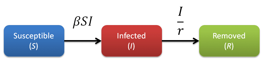
The rate of transfer from the Susceptible population to the Infected population is βSI, where β is the per-capita effective contact rate (C_e/N). The effective contact rate (C_e) is the number of effective contacts made by a given individual per unit time, where an effective contact is defined as a contact sufficient to lead to infection if it were to occur between a susceptible and an infectious individual. By practicing social distancing we are trying to reduce the value of β. The rate at which Infected individuals move into the Removed population is I/r, where r is the recovery delay. The recovery delay represents the length of time an individual remains infectious. The independent variable of the model is the time t, and the rates of change of the compartments are expressed as a set of differential equations [1]:

The basic reproduction number (R₀) is an indication of the transmissibility of a virus within a particular population. It represents the average number of new infections generated by an infected person in an entirely susceptible population. In this scheme R₀ is given by:

R₀ = βNr = C_er             (4)

where N is the total population:

N = S + I + R               (5)

This simple model predicts behavior similar to that observed in real-world epidemics [2]:

Implementation
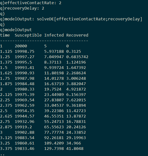
I first implement a function in kdb+ called solveDE which solves the above differential equations (1, 2, 3) numerically, and given a value for the effective contract rate and the recovery delay will return a table containing the quantity of each compartment at each time-step of the model.

Plotting the values of the three compartments at each time step gives the classic epidemic curve:

Figure 2 – Epidemic curve produced by SIR model

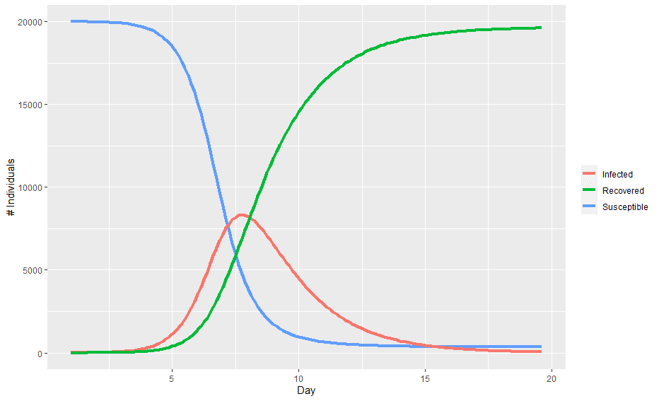
In the above chart, the population starts out entirely susceptible with a small number of infected individuals. As the infection spreads, the number of infected individuals accelerates before hitting a peak and then begins to decline as there are less and less individuals to infect.

Flattening the Curve
This model has two input parameters (the recovery delay and the effective contact rate), and we can use the model to study how their values influence the course of an epidemic.

In practice, there is little we can do to influence the recovery delay as this is mostly an intrinsic property of the virus. We can, however, influence the value of the second parameter – the effective contact rate. The global effort to reduce the effective contact rate through social distancing has become central to our lives in recent weeks. Experts have been urging us to practice social distancing in an effort to “flatten the curve”. If a virus spreads too quickly through a population, the initial surge of infections can exceed the capacity of our resource-limited healthcare systems, resulting in otherwise preventable deaths. The goal of “flattening the curve” is to spread the number of infections out over a longer period of time, thereby allowing healthcare systems to accommodate all individuals who become infected.

We can use the SIR model to simulate the effect of social distancing and observe the flattening of the infection curve. Use the slider to alter the value of the effective contact rate.

Model Calibration
A common task when working with models is to try and quantify model parameters that cannot easily be measured directly. A common approach to this problem is to adjust the model parameters until the model output closely matches empirical data. This approach is variously referred to as data-fitting, inverse modeling, or model calibration [3]. This approach can be used with models of infectious disease in order to estimate important epidemiological parameters such as R₀.  Early estimation of R₀ is crucial for strategy planning to mitigate and control an epidemic or pandemic caused by a novel infectious disease.

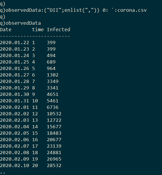
The goal here is to calibrate this model to empirical data from the COVID-19 outbreak in Wuhan in order to estimate R₀. The dataset I use was compiled by John Hopkins University [4]. It contains the number of confirmed cases of COVID-19 across globe between 2020.01.22 and 2020.03.09; however I limit this exercise to cases from Wuhan where the virus initially emerged. I first import the dataset into kdb+.

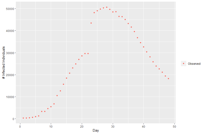
Plotting this data we can observe the infection curve:

Figure 3 – Infection curve – Wuhan (2020.01.22 – 2020.03.09)

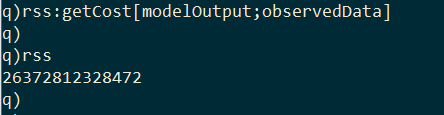
In order to calibrate the model, we need a way to compare how well the model output fits the empirical data. I implement a second kdb+ function called getCost, which takes the model output and the empirical data, and returns the residual sum of squares (RSS) between the observed and projected infection curves.

Now that we have a way to calculate the cost of a model, we can begin searching for the values of effective contact rate and recovery delay that produce the best-fit model. There are many ways of searching the parameter space, but here I take a Monte Carlo approach of using randomly sampled values.

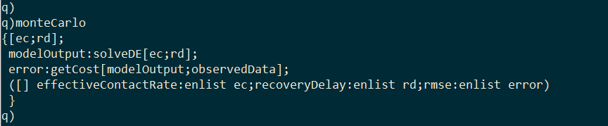
I wrap solveDE and getCost inside a third function called monteCarlo. Given values for effective contact rate and recovery delay, this function will generate the model output with solveDE, calculate the RSS of the output with getCost, and then return a single-rowed table containing the effective contact rate, the recovery delay, and the associated RSS.

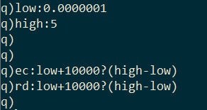
I generate 10,000 random values for effective contact rate and recovery delay within a range.

I pass these random values to the monteCarlo function in pairs using the each-both iterator and combine the results together with the built-in raze function.

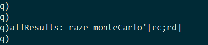
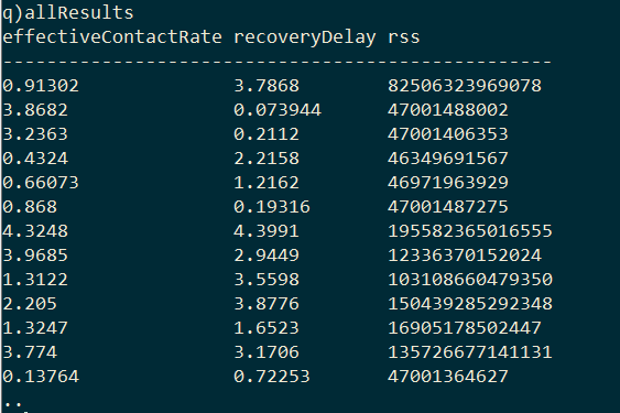
The result is a table with the pairs of model parameters and the RSS of the model they produced.

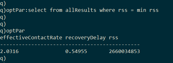
The optimal model parameters can then be found by selecting the row with the minimum RSS.

As I final step we can generate the optimal model by passing the optimized parameters to solveDE.

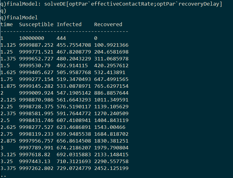
Plotting the model’s predicted infection curve over the real infection curve from Wuhan we can see that the model fits relatively well.

Figure 4 – Projected and observed infection curves

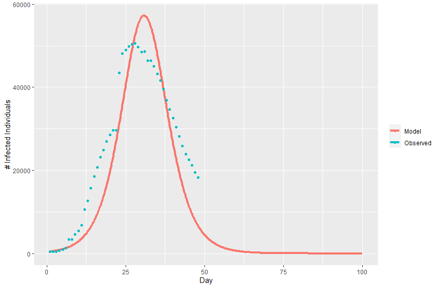
With optimized values for effective contact rate (2.0316) and recovery delay (0.54955), we can plug these values into equation (4)  to estimate the basic reproduction number (R₀ = 1.1165). This estimate of R₀ is on the low side of published estimates, with the World Health Organization estimating an R₀ between 1.4 and 2.5 [6]. It’s likely that the incidence data used here is under-reported. Additionally, the basic SIR model doesn’t take into account interventions that have taken place that would reduce the infection curve.

Conclusion

• We can analyze the dynamics of an epidemic using a simple SIR model.
• We can estimate key epidemiological parameters by fitting the model to empirical data.
• R₀ is a property of both the virus and the population. We can influence the value of the effective contact rate by practicing social distancing and thereby reduce R₀.

 

References:

[1] Duggan, J. 2016. System Dynamics Modeling with R. Springer

[2] Vynnycky, E. and White, R., 2010. An introduction to infectious disease modelling. OUP oxford.

[3] Schittkowski, K. 2013. Numerical data fitting in dynamical systems: a practical introduction with applications and software. Springer Science & Business Media.

[4] https://github.com/CSSEGISandData/COVID-19

[5] Kermack, W.O. and McKendrick, A.G. 1927. A contribution to the mathematical theory of epidemics. Proceedings of the Royal Society of London A: mathematical, physical and engineering sciences (1927), 700–721.

[6] Liu, Y., Gayle, A A., Wilder-Smith, A., Rocklöv, J. (2020) The reproductive number of COVID-19 is higher compared to SARS. Journal of Travel Medicine.