

Key Takeaways
- kdb+ is engineered for ultra-low latency and high-throughput environments
- Combining kdb+ with natural language capability democratizes complex query creation.
- Automating visualizations can be achieved via a simple function or using tools such as pandas-ai
In finance, billion-row time series datasets are common, which is why financial institutions have long trusted kdb+, the world’s fastest time series database for mission-critical workloads. Unlike traditional solutions, which move data to external tools for processing, kdb+ executes queries directly using its vectorized language, q. This minimizes latency and avoids the overhead of data movement, but can require careful planning and specialist skills when crafting complex queries.
In this blog, I will demonstrate how to democratize this process, combining kdb+ and PyKX (KX’s Python interface for kdb+) with natural language understanding to accelerate time to value.
I’ll show you how to:
- Import millions of rows into a kdb+ table
- Generate queries via an LLM
- Convert returned data frames to pandas
- Create a plot function
If you’d like to follow along, you can do so via my colab notebook.
Let’s begin.
Data ingestion
To begin, we will install a free personal license of PyKX (KX’s Python interface for kdb+). Then, for simplicity and convenience, ingest a sample stock dataset containing 3 million minute-level time-series records.
import pykx as kx
# Load a sample CSV and push it into q as 'trades'
pandas_tbl = pd.read_csv(
    'https://huggingface.co/datasets/opensporks/stocks/resolve/main/stocks.csv',
    parse_dates=['timestamp']
)
tbl = kx.toq(pandas_tbl)        # DataFrame → q Table
tbl = tbl.rename(columns={"close": "closePrice"})
kx.q['trades'] = tbl             # assign to q global
Let’s examine the results:
# get table description and save as text stored in a variable:
table_desc = tbl.dtypes
print(table_desc)

# get min and last date
min_date = kx.q('first trades`timestamp').pd()
max_date = kx.q('last trades`timestamp').pd()

print(f"\nMinimum timestamp: {min_date}")
print(f"Maximum timestamp: {max_date}")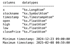
As you can see from the output, tickers, floats, and timestamps are returned.
Natural language translation
Next, we’ll create a translator that converts plain English questions into qSQL queries. I’m using this method because LLMs are not yet fully proficient in writing q, kdb+’s native query language. However, with qSQL being somewhat ANSI compliant, we can overcome this limitation by prompting our LLM with the subtle differences.
SYSTEM_PROMPT = 'Create a valid sql query based on this table schema and natural language query'

class TranslateResponse(BaseModel):
    qsql: str

def translate_to_qsql(nl_query: str, table: str, schema: str) -> str:
    system = (
        SYSTEM_PROMPT
    )
    user = (
        f"Table: {table}\n"
        f"Schema: {schema}\n"
        f"Question: {nl_query}"
    )
    resp = client.beta.chat.completions.parse(
        model="o3",
        messages=[
            {"role": "system", "content": system},
            {"role": "user",   "content": user},
        ],
        response_format=TranslateResponse,
    )
    return resp.parsed.qsql
Our system prompt now contains detailed instructions about the qSQL syntax and best practices. This will ensure valid and efficient queries for kdb+. This is very much a work in progress, so I welcome any feedback or suggestions from community members.
Automated visualization
When queries are processed and returned, we’ll want AI to generate the appropriate visualization based on their associated data structures. In this instance, I have created my own visualization function; however, you might also consider using pandas-ai, which is a more robust and feature-rich solution.
def visualize_df_with_plotly(df, model="gpt-4o", sample_size=20, temperature=0):
    """
    Given a pandas DataFrame df and an OpenAI-compatible client,
    infers a schema and sample, asks the model to generate Plotly Express code,
    and then executes and displays the resulting chart.
    """
    # 1. Build schema and sample, converting timestamps to strings
    sample_df = df.head(sample_size).copy()
    for col, dtype in sample_df.dtypes.items():
        if "datetime" in str(dtype).lower() or "timestamp" in str(dtype).lower():
            sample_df[col] = sample_df[col].astype(str)
    sample = sample_df.to_dict(orient="list")
    schema_auto = {col: str(dtype) for col, dtype in df.dtypes.items()}

# 2. Prepare prompts
    system = (
        "You're an expert Python data-visualizer. "
        "Given a DataFrame schema and sample data, "
        "write self-contained code using Plotly Express that "
        "takes the df and, creates a fig named fig, "
        "Write code that assigns df to fig, "
        "but do not call fig.show(). I will handle displaying. "
        "Feel free to show any other aggregations and print as numbers as you feel is needed as long as the figure is made"
        "GIVE ME ONLY CODE AND NOTHING ELSE."
        "Do not rewrite the values in the df, assume it is global in a dataframe called df"
        "Think about what the user wants in the query and provide it"
        "Never hardcode values"
    )
    user = (
        f"Schema: {json.dumps(schema_auto)}\n\n"
        f"Sample data: {json.dumps(sample, default=str)}"
    )
    # 3. Call the chat completion API
    resp = client.chat.completions.create(
        model=model,
        messages=[
            {"role": "system", "content": system},
            {"role": "user",   "content": user}
        ],
        temperature=temperature,
    )
    # 4. Extract the code from the response
    chart_code = resp.choices[0].message.content
    if chart_code.startswith("```"):
        chart_code = chart_code.split("\n", 1)[1].rsplit("\n```", 1)[0]
    print(chart_code)
    # 5. Execute the generated code
    local_vars = {"df": df, "px": px}
    exec(chart_code, {}, local_vars)
    # 6. Display the figure
    fig = local_vars.get("fig")
    if fig:
        fig.show()
    else:
        raise RuntimeError("The generated code did not produce a fig object.")
Plotting
Finally, we will combine everything into a powerful new function named query_and_plot, which will enable plot outputs to be generated from a natural language query.
def query_and_plot(nl_query: str, table: str = "trades") -> None:
    """
    Given a natural-language question about the kdb+ table,
    translates it to q-SQL, runs it, and renders an appropriate chart.
    """
    # --- translate to q-SQL ---
    # derive schema from the table in q
    q_tbl = tbl
    schema = str(q_tbl.dtypes)
    print(schema)

    # call the existing translator (assumes translate_to_qsql is defined globally)
    qsql = translate_to_qsql(nl_query, table, schema)
    print("🔧 Generated q-SQL:\n", qsql)
    # --- execute query ---
    result = kx.q.sql(qsql)
    df = result.pd()
    print("Resulting df After AI Query")
    display(df.head())
    print("\n── Resulting df Description ──")
    display(df.describe(include="all"))
    visualize_df_with_plotly(df)
Real-world testing
Let’s now test the solution with some real-world examples. Remember, LLMs can experience inconsistent outputs, meaning results may differ.
Example 1: Cumulative returns
To begin, I will ask the agent to chart the cumulative returns for both Tesla (TSLA) and Apple (AAPL).
query_and_plot("Chart the cumulative returns for TSLA and AAPL")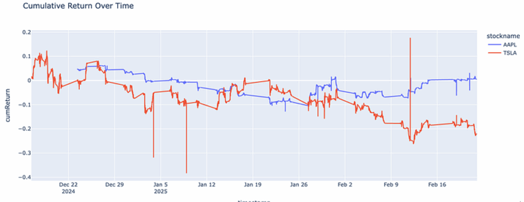
What this generates:
- A q-SQL query that calculates cumulative returns
- A multi-line chart showing performance over time
It also automatically handles date parsing and percentage calculations.
Example 2: Statistical analysis
Next, I will ask the agent to calculate the average price of each stock in our dataset.
query_and_plot("what is the average price for each stock?"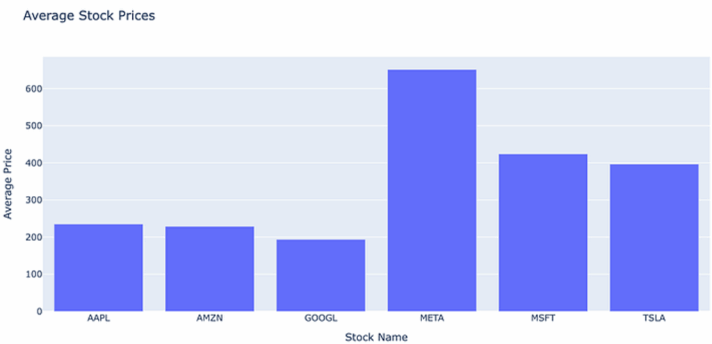
We can also ask which date had the highest closing price for each.
query_and_plot("Which day had the highest closing price for each stock?")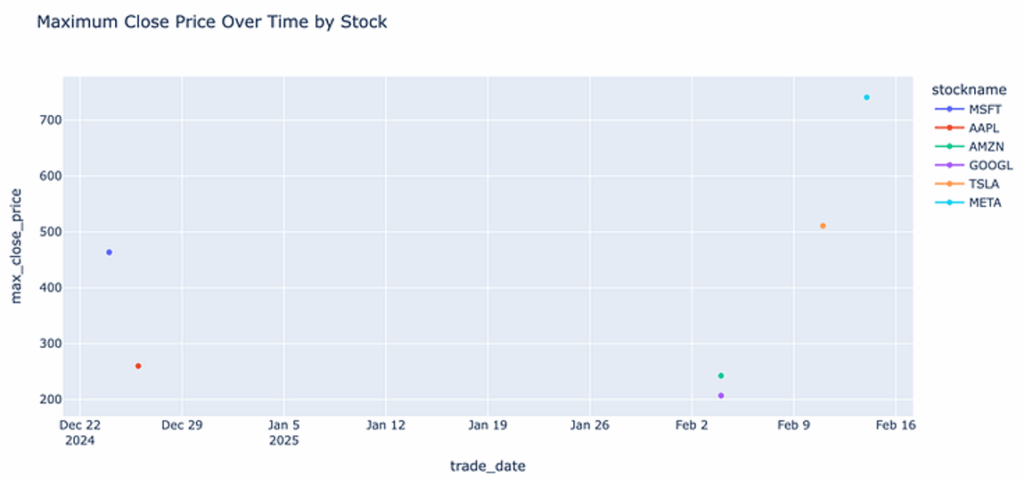
What this generates:
- A grouping query to calculate averages by stock symbol
- An appropriate bar chart or table visualization
- Clear labelling and formatting
By combining kdb+’s performance with AI’s natural language capabilities, we not only create a powerful tool for time series analysis but also democratize complex query building to anyone who can communicate in plain English. Both serve to enhance decision-making and accelerate new possibilities for innovation and growth.
If you enjoyed this blog, please check out my others on kx.com and connect with me on Slack. You can also find all of the code used in this blog via my colab notebook.