By Fionnuala Carr
As part of KX25, the international kdb+ user conference held May 18th in New York City, a series of seven JuypterQ notebooks were released and are now available on https://code.kx.com/q/ml/. Each notebook demonstrates how to implement a different machine learning technique in kdb+, primarily using embedPy, to solve all kinds of machine learning problems, from feature extraction to fitting and testing a model.
These notebooks act as a foundation to our users, allowing them to manipulate the code and get access to the exciting world of machine learning within KX. (For more about the KX machine learning team please watch Andrew Wilson’s presentation at KX25 on the KX Youtube channel).
Background
One of the simplest decision procedures that can be used for data classification is the nearest neighbor (NN) rule. It classifies a sample based on the category or class of its nearest neighbor. The NN-based classifiers use some or all of the patterns available in the training set to classify a test pattern. At its most basic these classifiers essentially involve finding the similarity between the test pattern and every pattern in the training set.
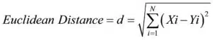
The k-Nearest Neighbors (k-NN) algorithm is a simple but effective algorithm, used for supervised classification and regression problems. KNN is a non-parametric, lazy learning algorithm which means that it doesn’t make any assumptions on the underlying data distribution and also that there is no explicit training phase. This is an advantage because in the real world most datasets don’t follow a derived distribution. The algorithm forms a majority vote between the k most similar instances to a given “unseen” observation. It iterates through the whole dataset computing the distance between the unseen observation and each training observation. There are many different distance metrics that can be used but the most popular choice is the Euclidean distance given by:
The algorithm then selects the k entries in the training set that is closest to the unseen observation. A label is given to that observation by finding the most common classification of these entries.
The dataset that will be used in this notebook is the UCI Breast Cancer Wisconsin (Diagnostics) dataset. It consists of 569 patients with 30 different features and they were classified if they were malignant or benign. The features in the dataset describe the characteristics of the cell nuclei present in the breast mass. Ten features are computed for each cell nucleus which include the radius, texture and perimeter.
Technical description
This notebook demonstrates the use of embedPy to import Python machine learning libraries such as scikit-learn and matplotlib which are used to import and analyze the breast cancer dataset. Two q scripts are loaded in which consist of general machine learning functions that are created in raw q and plotting functions that use matplotlib.
Firstly we investigate the dataset using q in which we check the shape of the dataset, if there are any missing values present and if the classes are balanced. This allows us to get insights into the dataset and informs us what necessary steps are to take before we apply the data to the k-Nearest Neighbors classifier. From this analysis, we can see that the classes are quite unbalanced which means that you could get a high accuracy of classifying if a patient had cancer or not without actually applying a classifier on the dataset.
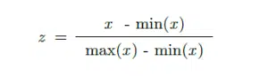
As the kNN classifier requires us to calculate the distance between points in the feature space, we inspected the range of the features. The ranges of features were calculated using the range function which is in native q and can be found in func.q . Matplotlib was imported using embedPy and a bar chart was created to visualize the ranges of the features. It was quite clear that there are large variations in the ranges of features and that the ranges needed to be standardized so that they were all on the same scale. Otherwise, the feature with the most magnified scale will get the highest weighting in terms of prediction. The min max scaling algorithm was used to scale each feature individually into a range 0-1 with the formula given below.
After preprocessing the dataset, the dataset is split into training and testing sets using the traintestsplit function that can be found in func.q. The next step is to find the optimal k value which gives the highest accuracy. We fit a kNN classifier with k values from 1 to 200 and evaluate the classifier’s accuracy. Using embedPy, the kNN classifier from scikit-learn is imported. The distance that the classifier uses is the minkowski distance with p=2 which is equivalent to the standard Euclidean metric. We apply the classifier to the dataset and store the predictions as kdb+ data. Using these predictions we can find the accuracy of the classifier using a q function that is defined in func.q. These accuracies are stored and plotted using matplotlib. From the plot, it can be seen that the accuracy increases up to a specific value of k and decreases after that value. It can be assumed that the model is overfitting for low values of k and underfitting for high values of k.
This technique is often referred to as hyperparameter tuning. Hyperparameters are parameters that define the models architecture. With applying a classifier such as kNN, it’s quite difficult to know what is the optimal k value. You can think of the k value as controlling the shape of the decision boundary which is used to classify new data points. The optimal k value can be said to produce the classifier with the highest accuracy. For this dataset, we find that the optimal k value is 11 as the accuracy score starts to decrease after this value.
If you would like to further investigate the uses of a kNN classifier, check out ML 03 K-Nearest Neighbors notebook on GitHub (https://code.kx.com/q/ml/). For more about kdb+ and kNN, please also refer to a previous KX blog on k-Nearest Neighbor with an accompanying whitepaper.
If you would like to try this, you can use Anaconda to integrate into your Python installation to set up your machine learning environment, or you can build your own, which consists of downloading kdb+, embedPy and JupyterQ. Look for installation steps on code.kx.com/q/ml/setup/.
Don’t hesitate to contact ai@kx.com if you have any suggestions or queries.
Other articles in this JupyterQ series of blogs by the KX Machine Learning Team:
Natural Language Processing in kdb+ by Fionnuala Carr
Neural Networks in kdb+ by Esperanza López Aguilera
Dimensionality Reduction in kdb+ by Conor McCarthy
Feature Engineering in kdb+ by Fionnuala Carr
Decision Trees in kdb+ by Conor McCarthy
Random Forests in kdb+ by Esperanza López Aguilera
Reference
N.S.Altman. An Introduction to Kernel and Nearest-Neighbor Nonparametric Regression. Available at https://www.tandfonline.com/doi/abs/10.1080/00031305.1992.10475879
Cahsai, A., Anagnostopoulos, C. , Ntarmos, N. and Triantafillou, P. (2017) Scaling k-Nearest Neighbors Queries (The Right Way). In: 2017 IEEE 37th International Conference on Distributed Computing Systems (ICDCS), Atlanta, GA, USA, 5-8 June 2017, pp. 1419-1430. ISBN 9781538617939. Available at: http://eprints.gla.ac.uk/138493/
Murty, M. and Devi, V. Nearest Neighbour Based Classifiers. In Pattern Recogition. 48-55. Springer Publishers 2011. Available at: https://link.springer.com/chapter/10.1007/978-0-85729-495-1_3
Friedman, J. H., F. Baskett and L. J. Shustek. An algorithm for finding nearest neighbours. IEEE Trans on Computers C-24(10): 1000–1006. 1975. Avaliable at: http://inspirehep.net/record/91686/files/slac-pub-1448.pdf
Patrick, E. A., and F. P. Fischer. A generalized k nearest neighbor rule. Information and Control 16: 128–152. 1970. Available at: https://www.sciencedirect.com/science/article/pii/S0019995870900811
Yunck, Thomas P. A technique to identify nearest neighbours. IEEE Trans. SMC SMC-6(10): 678–683. 1976. Available at: https://ieeexplore.ieee.org/abstract/document/4309418/


